RTG Command Reference
This chapter describes RTG commands with a generic description of parameter options and usage. This section also includes expected operation and output results.
Command line interface (CLI)
RTG is installed as a single executable in any system subdirectory where permissions authorize a particular community of users to run the application. RTG commands are executed through the RTG command-line interface (CLI). Each command has its own set of parameters and options described in this section.
Results are organized in results directories defined by command
parameters and settings. The command line shell environment should
include a set of familiar text post-processing tools, such as grep,
awk, or perl. Otherwise, no additional applications such as
databases or directory services are required.
RTG command syntax
Usage:
rtg COMMAND [OPTIONS] <REQUIRED>
To run an RTG command at the command prompt (either DOS window or Unix terminal), type the product name followed by the command and all required and optional parameters. For example:
$ rtg format -o human_REF_SDF human_REF.fasta
Typically results are written to output files specified with the -o
option. There is no default filename or filename extension added to
commands requiring specification of an output directory or format.
Many times, unfiltered output files are very large; the built-in
compression option generates block compressed output files with the
.gz extension automatically unless the parameter -Z or --no-gzip
is issued with the command.
Many command parameters require user-supplied information of various types, as shown in the following:
Type |
Description |
|---|---|
DIR, FILE |
File or directory name(s) |
SDF |
Sequence data that has been formatted to SDF |
INT |
Integer value |
FLOAT |
Floating point decimal value |
STRING |
A sequence of characters for comments, filenames, or labels |
REGION |
A genomic region specification (see below) |
Genomic region parameters take one of the following forms:
sequence_name (e.g.:
chr21) corresponds to the entirety of the named sequence.sequence_name:start (e.g.:
chr21:100000) corresponds to a single position on the named sequence.sequence_name:start-end (e.g.:
chr21:100000-110000) corresponds to a range that extends from the specified start position to the specified end position (inclusive). The positions are 1-based.sequence_name:position+length (e.g.:
chr21:100000+10000) corresponds to a range that extends from the specified start position that includes the specified number of nucleotides.sequence_name:position~padding (e.g.:
chr21:100000~10000) corresponds to a range that spans the specified position by the specified amount of padding on either side.
To display all parameters and syntax associated with an RTG command,
enter the command and type --help. For example: all parameters
available for the RTG format command are displayed when rtg format
--help is executed, the output of which is shown below.
Usage: rtg format [OPTION]... -o SDF FILE+
                  [OPTION]... -o SDF -I FILE
                  [OPTION]... -o SDF -l FILE -r FILE

Converts the contents of sequence data files (FASTA/FASTQ/SAM/BAM) into the RTG
Sequence Data File (SDF) format.

File Input/Output
  -f, --format=FORMAT            format of input. Allowed values are [fasta,
                                 fastq, sam-se, sam-pe, cg-fastq, cg-sam]
                                 (Default is fasta)
  -I, --input-list-file=FILE     file containing a list of input read files (1
                                 per line)
  -l, --left=FILE                left input file for FASTA/FASTQ paired end
                                 data
  -o, --output=SDF               name of output SDF
  -p, --protein                  input is protein. If this option is not
                                 specified, then the input is assumed to
                                 consist of nucleotides
  -q, --quality-format=FORMAT    format of quality data for fastq files (use
                                 sanger for Illumina 1.8+). Allowed values are
                                 [sanger, solexa, illumina]
  -r, --right=FILE               right input file for FASTA/FASTQ paired end
                                 data
      FILE+                      input sequence files. May be specified 0 or
                                 more times

Filtering
      --duster                   treat lower case residues as unknowns
      --exclude=STRING           exclude input sequences based on their name.
                                 If the input sequence contains the specified
                                 string then that sequence is excluded from the
                                 SDF. May be specified 0 or more times
      --select-read-group=STRING when formatting from SAM/BAM input, only
                                 include reads with this read group ID
      --trim-threshold=INT       trim read ends to maximise base quality above
                                 the given threshold

Utility
      --allow-duplicate-names    disable checking for duplicate sequence names
  -h, --help                     print help on command-line flag usage
      --no-names                 do not include name data in the SDF output
      --no-quality               do not include quality data in the SDF output
      --sam-rg=STRING|FILE       file containing a single valid read group SAM
                                 header line or a string in the form
                                 "@RG\tID:READGROUP1\tSM:BACT_SAMPLE\tPL:ILLUMINA"
Required parameters are indicated in the usage display; optional parameters are listed immediately below the usage information in organized categories.
Use the double-dash when typing the full-word command option, as in
--output:
$ rtg format --output human_REF_SDF human_REF.fasta
Commonly used command options provide an abbreviated single-character
version of a full command parameter, indicated with only a single dash,
(Thus --output is the same as specifying the command option with the
abbreviated character -o):
$ rtg format -o human_REF human_REF.fasta
A set of utility commands are provided through the CLI: version,
license, and help. Start with these commands to familiarize yourself
with the software.
The rtg version command invokes the RTG software and triggers the
launch of RTG product commands, options, and utilities:
$ rtg version
It will display the version of the RTG software installed, RAM requirements, for example:
$rtg version
Product: RTG Core 3.5
Core Version: 6236f4e (2014-10-31)
RAM: 40.0GB of 47.0GB RAM can be used by rtg (84%)
License: No license file required
Contact: support@realtimegenomics.com

Patents / Patents pending:
US: 7,640,256, 13/129,329, 13/681,046, 13/681,215, 13/848,653,
13/925,704, 14/015,295, 13/971,654, 13/971,630, 14/564,810
UK: 1222923.3, 1222921.7, 1304502.6, 1311209.9, 1314888.7, 1314908.3
New Zealand: 626777, 626783, 615491, 614897, 614560
Australia: 2005255348, Singapore: 128254

Citation:
John G. Cleary, Ross Braithwaite, Kurt Gaastra, Brian S. Hilbush, Stuart
Inglis, Sean A. Irvine, Alan Jackson, Richard Littin, Sahar
Nohzadeh-Malakshah, Mehul Rathod, David Ware, Len Trigg, and Francisco
M. De La Vega. "Joint Variant and De Novo Mutation Identification on
Pedigrees from High-Throughput Sequencing Data." Journal of
Computational Biology. June 2014, 21(6): 405-419.
doi:10.1089/cmb.2014.0029.
(c) Real Time Genomics Inc, 2014
To see release status of commands you are licensed to use, type rtg license:
$rtg license
License: No license file required

    Command name    Licensed?  Release Level

Data formatting:
    format          Licensed   GA
    sdf2fasta       Licensed   GA
    sdf2fastq       Licensed   GA

Utility:
    bgzip           Licensed   GA
    index           Licensed   GA
    extract         Licensed   GA
    sdfstats        Licensed   GA
    sdfsubset       Licensed   GA
    sdfsubseq       Licensed   GA
    mendelian       Licensed   GA
    vcfstats        Licensed   GA
    vcfmerge        Licensed   GA
    vcffilter       Licensed   GA
    vcfannotate     Licensed   GA
    vcfsubset       Licensed   GA
    vcfeval         Licensed   GA
    pedfilter       Licensed   GA
    pedstats        Licensed   GA
    rocplot         Licensed   GA
    version         Licensed   GA
    license         Licensed   GA
    help            Licensed   GA
To display all commands and usage parameters available to use with your
license, type rtg help:
$ rtg help
Usage: rtg COMMAND [OPTION]...
       rtg RTG_MEM=16G COMMAND [OPTION]...  (e.g. to set maximum memory use to 16 GB)

Type ``rtg help COMMAND`` for help on a specific command. The
following commands are available:

Data formatting:
      format                 convert a FASTA file to SDF
      cg2sdf                 convert Complete Genomics reads to SDF
      sdf2fasta              convert SDF to FASTA
      sdf2fastq              convert SDF to FASTQ
      sdf2sam                convert SDF to SAM/BAM
Read mapping:
      map                    read mapping
      mapf                   read mapping for filtering purposes
      cgmap                  read mapping for Complete Genomics data
Protein search:
      mapx                   translated protein search
Assembly:
      assemble               assemble reads into long sequences
      addpacbio              add Pacific Biosciences reads to an assembly
Variant detection:
      calibrate              create calibration data from SAM/BAM files
      svprep                 prepare SAM/BAM files for sv analysis
      sv                     find structural variants
      discord                detect structural variant breakends using discordant reads
      coverage               calculate depth of coverage from SAM/BAM files
      snp                    call variants from SAM/BAM files
      family                 call variants for a family following Mendelian inheritance
      somatic                call variants for a tumor/normal pair
      population             call variants for multiple potentially-related individuals
      lineage                call de novo variants in a cell lineage
      avrbuild               AVR model builder
      avrpredict             run AVR on a VCF file
      cnv                    call CNVs from paired SAM/BAM files
Metagenomics:
      species                estimate species frequency in metagenomic samples
      similarity             calculate similarity matrix and nearest neighbor tree
Simulation:
      genomesim              generate simulated genome sequence
      cgsim                  generate simulated reads from a sequence
      readsim                generate simulated reads from a sequence
      readsimeval            evaluate accuracy of mapping simulated reads
      popsim                 generate a VCF containing simulated population variants
      samplesim              generate a VCF containing a genotype simulated from a population
      childsim               generate a VCF containing a genotype simulated as a child of two parents
      denovosim              generate a VCF containing a derived genotype containing de novo variants
      samplereplay           generate the genome corresponding to a sample genotype
      cnvsim                 generate a mutated genome by adding CNVs to a template
Utility:
      bgzip                  compress a file using block gzip
      index                  create a tabix index
      extract                extract data from a tabix indexed file
      sdfstats               print statistics about an SDF
      sdfsplit               split an SDF into multiple parts
      sdfsubset              extract a subset of an SDF into a new SDF
      sdfsubseq              extract a subsequence from an SDF as text
      sam2bam                convert SAM file to BAM file and create index
      sammerge               merge sorted SAM/BAM files
      samstats               print statistics about a SAM/BAM file
      samrename              rename read id to read name in SAM/BAM files
      mapxrename             rename read id to read name in mapx output files
      mendelian              check a multi-sample VCF for Mendelian consistency
      vcfstats               print statistics from about variants contained within a VCF file
      vcfmerge               merge single-sample VCF files into a single multi-sample VCF
      vcffilter              filter records within a VCF file
      vcfannotate            annotate variants within a VCF file
      vcfsubset              create a VCF file containing a subset of the original columns
      vcfeval                evaluate called variants for agreement with a baseline variant set
      pedfilter              filter and convert a pedigree file
      pedstats               print information about a pedigree file
      avrstats               print statistics about an AVR model
      rocplot                plot ROC curves from vcfeval ROC data files
      usageserver            run a local server for collecting RTG command usage information
      version                print version and license information
      license                print license information for all commands
      help                   print this screen or help for specified command
The help command will only list the commands at GA or beta release level.
To display help and syntax information for a specific command from the command line, type the command and then the –help option, as in:
$ rtg format --help
Note
The following commands are synonymous:
rtg help format and rtg format --help
See also
Refer to Installation and deployment for information about installing the RTG product executable.
Data Formatting Commands
format
Synopsis:
The format command converts the contents of sequence data files
(FASTA/FASTQ/SAM/BAM) into the RTG Sequence Data File (SDF) format. This
step ensures efficient processing of very large data sets, by organizing
the data into multiple binary files within a named directory. The same
SDF format is used for storing sequence data, whether it be genomic
reference, sequencing reads, protein sequences, etc.
Syntax:
Format one or more files specified from command line into a single SDF:
$ rtg format [OPTION] -o SDF FILE+
Format one or more files specified in a text file into a single SDF:
$ rtg format [OPTION] -o SDF -I FILE
Format mate pair reads into a single SDF:
$ rtg format [OPTION] -o SDF -l FILE -r FILE
Examples:
For FASTA (.fa) genome reference data:
$ rtg format -o maize_reference maize_chr*.fa
For FASTQ (.fq) sequence read data:
$ rtg format -f fastq -q sanger -o h1_reads -l h1_sample_left.fq -r h1_sample_right.fq
Parameters:
File Input/Output |
||
|---|---|---|
|
|
The format of the input file(s). Allowed values are [fasta, fastq, fastq-interleaved, sam-se, sam-pe] (Default is fasta). |
|
|
Specifies a file containing a list of sequence data files (one per line) to be converted into an SDF. |
|
|
The left input file for FASTA/FASTQ paired end data. |
|
|
The name of the output SDF. |
|
|
Set if the input consists of protein. If this option is not specified, then the input is assumed to consist of nucleotides. |
|
|
The format of the quality data for fastq format files. (Use sanger for Illumina1.8+). Allowed values are [sanger, solexa, illumina]. |
|
|
The right input file for FASTA/FASTQ paired end data. |
|
Specifies a sequence data file to be converted into an SDF. May be specified 0 or more times. |
|
Filtering |
||
|---|---|---|
|
Treat lower case residues as unknowns. |
|
|
Exclude individual input sequences based on their name. If the input sequence name contains the specified string then that sequence is excluded from the SDF. May be specified 0 or more times. |
|
|
Set to only include only reads with this read group ID when formatting from SAM/BAM files. |
|
|
Set to trim the read ends to maximise the base quality above the given threshold. |
|
Utility |
||
|---|---|---|
|
Set to disable duplicate name detection. |
|
|
|
Prints help on command-line flag usage. |
|
Do not include sequence names in the resulting SDF. |
|
|
Do not include sequence quality data in the resulting SDF. |
|
|
Specifies a file containing a single valid read group SAM header line or a string in the form |
|
Usage:
Formatting takes one or more input data files and creates a single SDF.
Specify the type of file to be converted, or allow default to FASTA
format. To aggregate multiple input data files, such as when formatting
a reference genome consisting of multiple chromosomes, list all files on
the command line or use the --input-list-file flag to specify a file
containing the list of files to process.
For input FASTA and FASTQ files which are compressed, they must have a
filename extension of .gz (for gzip compressed data) or .bz2 (for
bzip2 compressed data).
When formatting human reference genome data, it is recommended that the
resulting SDF be augmented with chromosome reference metadata, in order
to enable automatic sex-aware features during mapping and variant
calling. The format command will automatically recognize several
common human reference genomes and install a reference configuration
file. If your reference genome is not recognized, a configuration can be
manually adapted from one of the examples provided in the RTG
distribution and installed in the SDF directory. The reference
configuration is described in RTG reference file format.
When using FASTQ input files you must specify the quality format being
used as one of sanger, solexa or illumina. As of Illumina pipeline
version 1.8 and higher, quality values are encoded in Sanger format and
so should be formatted using --quality-format=sanger. Output from
earlier Illumina pipeline versions should be formatted using
--quality-format=illumina for Illumina pipeline versions starting with
1.3 and before 1.8, or --quality-format=solexa for Illumina pipeline
versions less than 1.3.
For FASTQ files that represent paired-end read data, indicate each side
respectively using the --left=FILE and --right=FILE flags.
Sometimes paired-end reads are represented in a single FASTQ file by
interleaving each side of the read. This type of input can be
formatted by specifying fastq-interleaved as the format type.
The mapx command maps translated DNA sequence data against a protein
reference. You must use the -p, --protein flag to format the protein
reference used by mapx.
Use the sam-se format for single end SAM/BAM input files and the
sam-pe format for paired end SAM/BAM input files. Note that if the
input SAM/BAM files are sorted in coordinate order (for example if they
have already been aligned to a reference), it is recommended that they
be shuffled before formatting, so that subsequent mapping is not biased
by processing reads in chromosome order. For example, a BAM file can be
shuffled using samtools collate as follows:
$ samtools collate -uOn 256 reads.bam tmp-prefix >reads_shuffled.bam
And this can be carried out on the fly during formatting using bash process redirection in order to reduce intermediate I/O, for example:
$ rtg format --format sam-pe <(samtools collate -uOn 256 reads.bam temp-prefix) ...
The SDF for a read set can contain a SAM read group which will be
automatically picked up from the input SAM/BAM files if they contain
only one read group. If the input SAM/BAM files contain multiple read
groups you must select a single read group from the SAM/BAM file to
format using the --select-read-group flag or specify a custom read
group with the --sam-rg flag. The --sam-rg flag can also be used to
add read group information to reads given in other input formats. The
SAM read group stored in an SDF will be automatically used during
mapping the reads it contains to provide tracking information in the
output BAM files.
The --trim-threshold flag can be used to trim poor quality read ends
from the input reads by inspecting base qualities from FASTQ input. If
and only if the quality of the final base of the read is less than the
threshold given, a new read length is found which maximizes the overall
quality of the retained bases using the following formula.
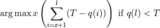
Where l is the original read length, x is the new read length, T is the given threshold quality and q(n) is the quality of the base at the position n of the read.
Note
Sequencing system read files and reference genome files often have the same extension and it may not always be obvious which file is a read set and which is a genome. Before formatting a sequencing system file, open it to see which type of file it is. For example:
$ less pf3.fa
In general, a read file typically begins with an @ or + character; a
genome reference file typically begins with the characters chr.
Normally when the input data contains multiple sequences with the same name the
format command will fail with an error. The --allow-duplicate-names flag
will disable this check conserving memory, but if the input data has multiple
sequences with the same name you will not be warned. Having duplicate sequence
names can cause problems with other commands, especially for reference data
since the output many commands identifies sequences by their names.
cg2sdf
Synopsis:
Converts Complete Genomics sequencing system reads to RTG SDF format.
Syntax:
Multi-file input specified from command line:
$ rtg cg2sdf [OPTION]... -o SDF FILE+
Multi-file input specified in a text file:
$ rtg cg2sdf [OPTION]... -o SDF -I FILE
Example:
$ rtg cg2sdf -I CG_source_files -o CG_reads
Parameters:
File Input/Output |
||
|---|---|---|
|
|
File containing a list of Complete Genomics TSV files (1 per line) |
|
|
Name of output SDF. |
|
File in Complete Genomics TSV format. May be specified 0 or more times. |
|
Filtering |
||
|---|---|---|
|
Maximum number of Ns allowed in either side for a read (Default is 5) |
|
Utility |
||
|---|---|---|
|
|
Print help on command-line flag usage. |
|
Does not include quality data in the resulting SDF. |
|
|
File containing a single valid read group SAM header line or a string in the form |
|
Usage:
The cg2sdf command converts Complete Genomics reads into an RTG SDF.
RTG supports two versions of Complete Genomics reads: the original 35 bp paired end read structure (“version 1”); and the newer 29 bp paired end structure (“version 2”). The 29 bp reads are sometimes equivalently represented as 30 bp with a redundant single base overlap containing an ‘N’ at position 20. This alternate representation is automatically normalised by RTG during processing.
The command accepts input files in the Complete Genomics read data
format entered at the command line. The reads for a single sample are
typically supplied in a large number of files. For consistent operation
with multiple samples, use the -I, --input-list-file flag to specify
a text file that lists all the files to format, specifying one filename
per line.
Using the --sam-rg flag the SDF for a read set can contain the SAM
read group specified. The SAM read group stored in an SDF will be
automatically used during mapping the reads it contains to provide
tracking information in the output BAM files. For version 1 reads, the
platform (PL) must be specified as COMPLETE, and for version 2
reads, the platform must be specified as COMPLETEGENOMICS.
Complete Genomics often produces “no calls” in the reads, represented by
multiple Ns. Sometimes, numerous Ns indicate a low quality read. The
--max-unknowns option limits how many Ns will be added to the SDF
during conversion. If there are more than the specified number of Ns in
one arm of the read, they read will not be added to the SDF.
sdf2cg
Synopsis:
Converts SDF formatted data into Complete Genomics TSV file(s).
Syntax:
Extract specific sequences listed on command line:
$ rtg sdf2cg [OPTION]... -i SDF -o FILE STRING+
Extract specific sequences listed in text file
$ rtg sdf2cg [OPTION]... -i SDF -o FILE -I FILE
Extract range of sequences by sequence id
$ rtg sdf2cg [OPTION]... -i SDF -o FILE --end-id INT --start-id INT
Parameters:
File Input/Output |
||
|---|---|---|
|
|
SDF containing sequences |
|
|
Output filename (extension added if not present). Use ‘-’ to write to standard output |
Filtering |
||
|---|---|---|
|
Exclusive upper bound on sequence id |
|
|
|
File containing sequence ids, or sequence names if –names flag is set, one per line |
|
|
Interpret supplied sequence as names instead of numeric ids |
|
Inclusive lower bound on sequence id |
|
|
ID of sequence to extract, or sequence name if –names flag is set. May be specified 0 or more times |
|
Utility |
||
|---|---|---|
|
|
Print help on command-line flag usage |
|
|
Maximum number of nucleotides to print on a line of output. A value of 0 indicates no limit (Default is 0) |
|
|
Do not gzip the output |
Usage:
The sdf2cg command converts RTG SDF data into Complete Genomics
reads format.
While any SDF data can be consumed by this command to produce a CG TSV file, real Complete Genomics data typically has specific read lengths and other characteristics that would make normal data fed through this command inappropriate for use in a Complete Genomics pipeline. However this command can be used to turn SDF formatted CG data back into TSV close to its original form.
See also
sdf2fasta
Synopsis:
Convert SDF data into a FASTA file.
Syntax:
$ rtg sdf2fasta [OPTION]... -i SDF -o FILE
Example:
$ rtg sdf2fasta -i humanSDF -o humanFASTA_return
Parameters:
File Input/Output |
||
|---|---|---|
|
|
SDF containing sequences. |
|
|
Output filename (extension added if not present). Use ‘-’ to write to standard output. |
Filtering |
||
|---|---|---|
|
Only output sequences with sequence id less than the given number. (Sequence ids start at 0). |
|
|
Only output sequences with sequence id greater than or equal to the given number. (Sequence ids start at 0). |
|
|
|
Name of a file containing a list of sequences to extract, one per line. |
|
Interpret any specified sequence as names instead of numeric sequence ids. |
|
|
Interpret any specified sequence as taxon ids instead of numeric sequence ids. This option only applies to a metagenomic reference species SDF. |
|
|
Specify one or more explicit sequences to extract, as sequence id, or sequence name if –names flag is set. |
|
Utility |
||
|---|---|---|
|
|
Prints help on command-line flag usage. |
|
Interleave paired data into a single output file. Default is to split to separate output files. |
|
|
|
Set the maximum number of nucleotides or amino acids to print on a line of FASTA output. Should be nonnegative, with a value of 0 indicating that the line length is not capped. (Default is 0). |
|
|
Set this flag to create the FASTA output file without compression. By default the output file is compressed with blocked gzip. |
Usage:
Use the sdf2fasta command to convert SDF data into FASTA format. By
default, sdf2fasta creates a separate line of FASTA output for each
sequence. These lines will be as long as the sequences themselves. To
make them more readable, use the -l, --line-length flag and define a
reasonable record length like 75.
By default all sequences will be extracted, but flags may be specified
to extract reads within a range, or explicitly specified reads (either
by numeric sequence id or by sequence name if --names is set).
Additionally, when the input SDF is a metagenomic species reference SDF,
the --taxons option, any supplied id is interpreted as a taxon id and
all sequences assigned directly to that taxon id will be output. This
provides a convenient way to extract all sequence data corresponding to
a single (or multiple) species from a metagenomic species reference SDF.
Sequence ids are numbered starting at 0, the --start-id flag is an inclusive
lower bound on id and the --end-id flag is an exclusive upper bound. For
example if you have an SDF with five sequences (ids: 0, 1, 2, 3, 4) the
following command:
$ rtg sdf2fasta --start-id=3 -i mySDF -o output
will extract sequences with id 3 and 4. The command:
$ rtg sdf2fasta --end-id=3 -i mySDF -o output
will extract sequences with id 0, 1, and 2. And the command:
$ rtg sdf2fasta --start-id=2 --end-id=4 -i mySDF -o output
will extract sequences with id 2 and 3.
sdf2fastq
Synopsis:
Convert SDF data into a FASTQ file.
Syntax:
$ rtg sdf2fastq [OPTION]... -i SDF -o FILE
Example:
$ rtg sdf2fastq -i humanSDF -o humanFASTQ_return
Parameters:
File Input/Output |
||
|---|---|---|
|
|
Specifies the SDF data to be converted. |
|
|
Specifies the file name used to write the resulting FASTQ output. |
Filtering |
||
|---|---|---|
|
Only output sequences with sequence id less than the given number. (Sequence ids start at 0). |
|
|
Only output sequences with sequence id greater than or equal to the given number. (Sequence ids start at 0). |
|
|
|
Name of a file containing a list of sequences to extract, one per line. |
|
Interpret any specified sequence as names instead of numeric sequence ids. |
|
|
Specify one or more explicit sequences to extract, as sequence id, or sequence name if –names flag is set. |
|
Utility |
||
|---|---|---|
|
|
Prints help on command-line flag usage. |
|
|
Set the default quality to use if the SDF does not contain sequence quality data (0-63). |
|
Interleave paired data into a single output file. Default is to split to separate output files. |
|
|
|
Set the maximum number of nucleotides or amino acids to print on a line of FASTQ output. Should be nonnegative, with a value of 0 indicating that the line length is not capped. (Default is 0). |
|
|
Set this flag to create the FASTQ output file without compression. By default the output file is compressed with blocked gzip. |
Usage:
Use the sdf2fastq command to convert SDF data into FASTQ format. If no
quality data is available in the SDF, use the -q, --default-quality
flag to set a quality score for the FASTQ output. The quality encoding
used during output is sanger quality encoding. By default, sdf2fastq
creates a separate line of FASTQ output for each sequence. As with
sdf2fasta, there is an option to use the -l, --line-length flag to
restrict the line lengths to improve readability of long sequences.
By default all sequences will be extracted, but flags may be specified
to extract reads within a range, or explicitly specified reads (either
by numeric sequence id or by sequence name if --names is set).
It may be preferable to extract data to unaligned SAM/BAM format using
sdf2sam, as this preserves read-group information stored in the SDF
and may also be more convenient when dealing with paired-end data.
The --start-id and --end-id flags behave as in sdf2fasta.
sdf2sam
Synopsis:
Convert SDF read data into unaligned SAM or BAM format file.
Syntax:
$ rtg sdf2sam [OPTION]... -i SDF -o FILE
Example:
$ rtg sdf2sam -i samplereadsSDF -o samplereads.bam
Parameters:
File Input/Output |
||
|---|---|---|
|
|
Specifies the SDF data to be converted. |
|
|
Specifies the file name used to write the resulting SAM/BAM to. The output format is automatically determined based on the filename specified. If ‘-’ is given, the data is written as uncompressed SAM to standard output. |
Filtering |
||
|---|---|---|
|
Only output sequences with sequence id less than the given number. (Sequence ids start at 0). |
|
|
Only output sequences with sequence id greater than or equal to the given number. (Sequence ids start at 0). |
|
|
|
Name of a file containing a list of sequences to extract, one per line. |
|
Interpret any specified sequence as names instead of numeric sequence ids. |
|
|
Specify one or more explicit sequences to extract, as sequence id, or sequence name if –names flag is set. |
|
Utility |
||
|---|---|---|
|
|
Prints help on command-line flag usage. |
|
|
Set this flag when creating SAM format output to disable compression. By default SAM is compressed with blocked gzip, and BAM is always compressed. |
Usage:
Use the sdf2sam command to convert SDF data into unaligned SAM/BAM
format. By default all sequences will be extracted, but flags may be
specified to extract reads within a range, or explicitly specified reads
(either by numeric sequence id or by sequence name if --names is set).
This command is a useful way to export paired-end data to a single
output file while retaining any read group information that may be
stored in the SDF.
The output format is either SAM/BAM depending on the specified output file name.
e.g. output.sam or output.sam.gz will output as SAM, whereas
output.bam will output as BAM. If neither SAM or BAM format is indicated by
the file name then BAM will be used and the output file name adjusted
accordingly. e.g output will become output.bam. However if standard
output is selected (-) then the output will always be in uncompressed SAM
format.
The --start-id and --end-if behave as in sdf2fasta.
fastqtrim
Synopsis:
Trim reads in FASTQ files.
Syntax:
$ rtg fastqtrim [OPTION]... -i FILE -o FILE
Example:
Apply hard base removal from the start of the read and quality-based trimming of terminal bases:
$ rtg fastqtrim -s 12 -E 18 -i S12_R1.fastq.gz -o S12_trimmed_R1.fastq.gz
Parameters:
File Input/Output |
||
|---|---|---|
|
|
Input FASTQ file, Use ‘-’ to read from standard input. |
|
|
Output filename. Use ‘-’ to write to standard output. |
|
|
Quality data encoding method used in FASTQ input files (Illumina 1.8+ uses sanger). Allowed values are [sanger, solexa, illumina] (Default is sanger) |
Filtering |
||
|---|---|---|
|
Discard reads that have zero length after trimming. Should not be used with paired-end data. |
|
|
|
Trim read ends to maximise base quality above the given threshold (Default is 0) |
|
If a read ends up shorter than this threshold it will be trimmed to zero length (Default is 0) |
|
|
|
Trim read starts to maximise base quality above the given threshold (Default is 0) |
|
|
Always trim the specified number of bases from read end (Default is 0) |
|
|
Always trim the specified number of bases from read start (Default is 0) |
Utility |
||
|---|---|---|
|
|
Print help on command-line flag usage. |
|
|
Do not gzip the output. |
|
|
If set, output in reverse complement. |
|
Seed used during subsampling. |
|
|
If set, subsample the input to retain this fraction of reads. |
|
|
|
Number of threads (Default is the number of available cores) |
Usage:
Use fastqtrim to apply custom trimming and preprocessing to raw
FASTQ files prior to mapping and alignment. The format command
contains some limited trimming options, which are applied to all input
files, however in some cases different or specific trimming operations
need to be applied to the various input files. For example, for
paired-end data, different trimming may need to be applied for the left
read files compared to the right read files. In these cases,
fastqtrim should be used to process the FASTQ files first.
The --end-quality-threshold flag can be used to trim poor quality bases
from the ends of the input reads by inspecting base qualities from FASTQ
input. If and only if the quality of the final base of the read is less
than the threshold given, a new read length is found which maximizes the
overall quality of the retained bases using the following formula:
where l is the original read length, x is the new read length, T
is the given threshold quality and q(n) is the quality of the base at
the position n of the read. Similarly, --start-quality-threshold
can be used to apply this quality-based thresholding to the start of
reads.
Some of the trimming options may result in reads that have no bases
remaining. By default, these are output as zero-length FASTQ reads,
which RTG commands are able to handle normally. It is also possible to
remove zero-length reads altogether from the output with the
--discard-empty-reads option, however this should not be used when
processing FASTQ files corresponding to paired-end data, otherwise the
pairs in the two files will no longer be matched.
Similarly, when using the --subsample option to down-sample a FASTQ
file for paired-end data, you should specify an explicit randomization
seed via --seed and use the same seed value for the left and right
files.
Formatting with filtering on the fly
Running custom filtering with fastqtrim need not mean that
additional disk space is required or that formatting be slowed down due
to additional disk I/O. It is possible when using standard unix shells
to perform the filtering on the fly. The following example demonstrates
how to apply different trimming options to left and right files while
formatting to SDF:
$ rtg format -f fastq -o S12_trimmed.sdf \
    -l <(rtg fastqtrim -s 12 -E 18 -i S12_R1.fastq.gz -o -)
    -r <(rtg fastqtrim -E 18 -i S12_R2.fastq.gz -o -)
See also
petrim
Synopsis:
Trim paired-end read FASTQ files based on read arm alignment overlap.
Syntax:
$ rtg petrim [OPTION]... -l FILE -o FILE -r FILE
Parameters:
File Input/Output |
||
|---|---|---|
|
|
Left input FASTQ file (AKA R1) |
|
|
Output filename prefix. Use ‘-’ to write to standard output. |
|
|
Quality data encoding method used in FASTQ input files (Illumina 1.8+ uses sanger). Allowed values are [sanger, solexa, illumina] (Default is sanger) |
|
|
Right input FASTQ file (AKA R2) |
Sensitivity Tuning |
||
|---|---|---|
|
Aligner indel band width scaling factor, fraction of read length allowed as an indel (Default is 0.5) |
|
|
Penalty for a gap extension during alignment (Default is 1) |
|
|
Penalty for a gap open during alignment (Default is 19) |
|
|
|
Minimum percent identity in overlap to trigger overlap trimming (Default is 90) |
|
|
Minimum number of bases in overlap to trigger overlap trimming (Default is 25) |
|
Penalty for a mismatch during alignment (Default is 9) |
|
|
Soft clip alignments if indels occur INT bp from either end (Default is 5) |
|
|
Penalty for unknown nucleotides during alignment (Default is 5) |
|
Filtering |
||
|---|---|---|
|
If set, discard pairs where both reads have zero length (after any trimming) |
|
|
If set, discard pairs where either read has zero length (after any trimming) |
|
|
Assume R1 starts with probes this long, and trim R2 bases that overlap into this (Default is 0) |
|
|
|
If set, merge overlapping reads at midpoint of overlap region. Result is in R1 (R2 will be empty) |
|
|
If set, trim overlapping reads to midpoint of overlap region. |
|
If a read ends up shorter than this threshold it will be trimmed to zero length (Default is 0) |
|
|
Method used to alter bases/qualities at mismatches within overlap region. Allowed values are [none, zero-phred, pick-best] (Default is none) |
|
|
Assume R2 starts with probes this long, and trim R1 bases that overlap into this (Default is 0) |
|
Utility |
||
|---|---|---|
|
|
Print help on command-line flag usage. |
|
Interleave paired data into a single output file. Default is to split to separate output files. |
|
|
|
Do not gzip the output. |
|
Seed used during subsampling. |
|
|
If set, subsample the input to retain this fraction of reads. |
|
|
|
Number of threads (Default is the number of available cores) |
Usage:
Paired-end read sequencing with read lengths that are long relative to the typical library fragment size can often result in the same bases being sequenced by both arms. This repeated sequencing of bases within the same fragment can skew variant calling, and so it can be advantageous to remove such read overlap.
In some cases, complete read-through can occur, resulting in additional adaptor or non-genomic bases being present at the ends of reads.
In addition, some library preparation methods rely on the ligation of
synthetic probe sequence to attract target DNA, which is subsequently
sequenced. Since these probe bases do not represent genomic material,
they must be removed at some point during the analytic pipeline prior to
variant calling, otherwise they could act as a reference bias when
calling variants. Removal from the primary arm where the probe is
attached is typically easy enough (e.g. via fastqtrim), however in
cases of high read overlap, probe sequence can also be present in the
other read arm.
petrim aligns each read arm against it’s mate with high stringency
in order to identify cases of read overlap. The sensitivity of read
overlap detection is primarily controlled through the use of
--min-identity and --min-overlap-length, although it is also
possible to adjust the penalties used during alignment.
The following types of trimming or merging may be applied.
Removal of non-genomic bases due to complete read-through. This removal is always applied.
Removal of overlap bases impinging into regions occupied by probe bases. For example, if the left arms contain 11-mer probes, using
--left-probe-length=11will result in the removal of any right arm bases that overlap into the first 11 bases of the left arm. Similar trimming is available for situations where probes are ligated to the right arm by using--right-probe-length.Adjustment of mismatching read bases inside areas of overlap. Such mismatches indicate that one or other of the bases has been incorrectly sequenced. Alteration of these bases is selected by supplying the
--mismatch-adjustmentflag with a value ofzero-phredto alter the phred quality score of both bases to zero, orpick-bestto choose whichever base had the higher reported quality score.Removal of overlap regions by trimming both arms back to a point where no overlap is present. An equal number of bases are removed from each arm. This trimming is enabled by specifying
--midpoint-trimand takes place after any read-through or probe related trimming.Merging non-redundant sequence from both reads to create a single read, enabled via
--midpoint-merge. This is like--midpoint-trimwith a subsequent moving of the R2 read onto the end of the the R1 read (thus the R2 read becomes empty).
After trimming or merging it is possible that one or both of the arms of
the pair have no bases remaining, and a strategy is needed to handle
these pairs. The default is to retain such pairs in the output, even if
one or both are zero-length. When both arms are zero-length, the pair
can be dropped from output with the use of --discard-empty-pairs. If
downstream processing cannot handle zero-length reads,
--discard-empty-reads will drop a read pair if either of the arms is
zero-length.
petrim also provides the ability to down-sample a read set by using
the --subsample option. This will produce a different sampling each time,
unless an explicit randomization seed is specified via --seed.
Formatting with paired-end trimming on the fly
Running custom filtering with petrim can be done in standard Unix
shells without incurring the use of additional disk space or unduly
slowing down the formatting of reads. The following example demonstrates
how to apply paired-end trimming while formatting to SDF:
$ rtg format -f fastq-interleaved -o S12_trimmed.sdf \
    <(rtg petrim -l S12_R1.fastq.gz -r S12_R2.fastq.gz -m -o - --interleaved)
This can even be combined with fastqtrim to provide extremely
flexible trimming:
$ rtg format -f fastq-interleaved -o S12_trimmed.sdf \
    <(rtg petrim -m -o - --interleave \
         -l <(rtg fastqtrim -s 12 -E 18 -i S12_R1.fastq.gz -o -) \
         -r <(rtg fastqtrim -E 18 -i S12_R2.fastq.gz -o -) \
     )
Note
petrim currently assumes Illumina paired-end sequencing,
and aligns the reads in FR orientation. Sequencing methods which
produce arms in a different orientation can be processed by first
converting the input files using fastqtrim --reverse-complement,
running petrim, followed by another fastqtrim
--reverse-complement to restore the reads to their original
orientation.
Read Mapping Commands
map
Synopsis:
The map command aligns sequence reads onto a reference genome,
creating an alignments file in the Sequence Alignment/Map (SAM) format.
It can be used to process single-end or paired-end reads, of equal or
variable length.
Syntax:
Map using an SDF or a single end sequence file:
$ rtg map [OPTION]... -o DIR -t SDF -i SDF|FILE
Map using paired end sequence files:
$ rtg map [OPTION]... -o DIR -t SDF -l FILE -r FILE
Example:
$ rtg map -t strain_REF -i strain_READS -o strain_MAP -b 2 -U
Parameters:
File Input/Output |
||
|---|---|---|
|
|
Input format for reads. Allowed values are [sdf, fasta, fastq, fastq-interleaved, sam-se, sam-pe] (Default is sdf) |
|
|
Input read set. |
|
|
Left input file for FASTA/FASTQ paired end reads. |
|
|
Directory for output. |
|
|
Quality data encoding method used in FASTQ input files (Illumina 1.8+ uses sanger). Allowed values are [sanger, solexa, illumina] (Default is sanger) |
|
|
Right input file for FASTA/FASTQ paired end reads. |
|
Output the alignment files in SAM format. |
|
|
|
SDF containing template to map against. |
Sensitivity Tuning |
||
|---|---|---|
|
Set the fraction of the read length that is allowed to be an indel. Decreasing this factor will allow faster processing, at the expense of only allowing shorter indels to be aligned. (Default is 0.5). |
|
|
Set the aligner mode to be used. Allowed values are [auto, table, general] (Default is auto). |
|
|
Restrict calibration to mappings falling within the regions in the supplied BED file. |
|
|
filter k-mers that occur more than this many times in the reference using a blacklist |
|
|
Set the penalty for extending a gap during alignment. (Default is 1). |
|
|
Set the penalty for a gap open during alignment. (Default is 19). |
|
|
|
Guarantees number of positions that will be detected in a single indel. For example, -c 3 specifies 3 nucleotide insertions or deletions. (Default is 1). |
|
|
Guarantees minimum number of indels which will be detected when used with read less than 64 bp long. For example -b 1 specifies 1 insertion or deletion. (Default is 1). |
|
|
The maximum permitted fragment size when mating paired reads. (Default is 1000). |
|
|
The minimum permitted fragment size when mating paired reads. (Default is 0). |
|
Set the penalty for a mismatch during alignment. (Default is 9). |
|
|
|
Set the orientation required for proper pairs. Allowed values are [fr, rf, tandem, any] (Default is any). |
|
Genome relationships pedigree containing sex of sample. |
|
|
Where INT specifies the percentage of all hashes to keep, discarding the remaining percentage of the most frequent hashes. Increasing this value will improve the ability to map sequences in repetitive regions at a cost of run time. It is also possible to specify the option as an absolute count (by omitting the percent symbol) where any hash exceeding the threshold will be discarded from the index. (Default is 90%). |
|
|
Specifies the sex of the individual. Allowed values are [male, female, either]. |
|
|
Set to soft clip alignments when an indel occurs within that many nucleotides from either end of the read. (Default is 5). |
|
|
|
Set the step size. (Default is word size). |
|
|
Guarantees minimum number of substitutions to be detected when used with read data less than 64 bp long. (Default is 1). |
|
Set the penalty for unknown nucleotides during alignment. (Default is 5). |
|
|
|
Specifies an internal minimum word size used during the initial matching phase. Word size selection optimizes the number of reads for a desired level of sensitivity (allowed mismatches and indels) given an acceptable alignment speed. (Default is 22, or read length / 2, whichever is smaller). |
Filtering |
||
|---|---|---|
|
Only map sequences with sequence id less than the given number. (Sequence ids start at 0). |
|
|
Only map sequences with sequence id greater than or equal to the given number. (Sequence ids start at 0). |
|
Reporting |
||
|---|---|---|
|
Output all alignments meeting thresholds instead of applying mating and N limits. |
|
|
The maximum mismatches for mappings across mated results, alias for |
|
|
|
The maximum mismatches for mappings in single-end mode (as absolute value or percentage of read length). (Default is 10%). |
|
|
Sets the maximum number of reported mapping results (locations) per read when it maps to multiple locations with the same alignment score (AS). Allowed values are between 1 and 255. (Default is 5). |
|
|
The maximum mismatches for mappings of unmated results (as absolute value or percentage of read length). (Default is 10%). |
|
Specifies a file containing a single valid read group SAM header line or a string in the form |
|
|
If set, will only output a single random top hit for each read. |
|
Utility |
||
|---|---|---|
|
|
Prints help on command-line flag usage. |
|
Produce cigars in legacy format (using M instead of X or =) in SAM/BAM output. When set will also produce the MD field. |
|
|
Set this flag to not produce the calibration output files. |
|
|
|
Set this flag to create the SAM output files without compression. By default the output files are compressed with tabix compatible blocked gzip. |
|
Set to output mated, unmated and unmapped alignment records into separate SAM/BAM files. |
|
|
Do not perform structural variant processing. |
|
|
Do not output unmapped reads. Some reads that map multiple times will not be aligned, and are reported as unmapped. These reads are reported with XC attributes that indicate the reason they were not mapped. |
|
|
Do not output unmated reads when in paired-end mode. |
|
|
Output read names instead of sequence ids in SAM/BAM files. (Uses more RAM). |
|
|
Set the directory to use for temporary files during processing. (Defaults to output directory). |
|
|
|
Specify the number of threads to use in a multi-core processor. (Default is all available cores). |
Usage:
The map command locates reads against a reference using an indexed
search method, aligns reads at each location, and then reports
alignments within a threshold as a record in a BAM file. Some extensions
have been made to the output format. Please consult
SAM/BAM file extensions (RTG map command output) for more information.
By default the alignment records will be output into a single BAM format
file called alignments.bam. When the --sam flag is set it will
instead be output in compressed SAM format to a file called
alignments.sam.gz.
When using the --no-merge flag the output will be put into separate
files for mated, unmated and unmapped records depending on the kind of
reads being mapped. When mapping single end reads it will produce a
single output file containing the mappings called alignments.bam. When
mapping paired end reads it will produce two files, mated.bam with
paired alignments and unmated.bam with unpaired alignments. A file
containing the unmapped reads called unmapped.bam is also produced in
both cases. When used in conjunction with the --sam flag each of the
separate files will be in compressed SAM format rather than BAM format.
It is highly recommended to ensure that read group tracking information
is present in the output BAM files. When mapping directly from a SAM/BAM
file with a single read group, or from an SDF with the read group
information stored this is automatically set and does not need to be set
manually. This read group information can also be explicitly supplied by
using the --sam-rg flag to provide a SAM-formatted read group header
line. The header should specify at least the ID, SM and PL fields
for the read group. For more details see Using SAM/BAM Read Groups in RTG map.
During mapping RTG automatically creates a calibration file alongside
each BAM file containing information about base qualities, average
coverage levels etc. This calibration information is utilized during
variant calling to give more accurate results and to determine when
coverage levels are abnormally high. When processing exome data, it is
important that this calibration information should only be computed for
mappings within the exome capture regions, using the --bed-regions
flag to give the name of a bed file containing your vendor-supplied
exome capture regions, otherwise the computed coverage levels will be
much lower than actual and subsequent variant calling will be
affected. Calibration computation is disabled when read group
information is not present. If you decide to merge BAM files, it is
recommended that you use the sammerge command, as this is aware of
the calibration files and will ensure that the calibration information
is preserved through the merge process. Calibration information can also
be explicitly regenerated for a BAM file by using the calibrate
command.
Alignments are measured with an alignment score where each match adds 0,
each mismatch (substitution) adds --mismatch-penalty (default 9), each
gap (insertion or deletion) adds --gap-open-penalty (default 19), and
each gap extension adds --gap-extend-penalty (default 1). For more
information about alignment scoring see Alignment scoring.
The --aligner-band-width parameter controls the size of indels that
can be aligned. It represents the fraction of the read length that can
be aligned as an indel. Decreasing this factor will allow faster
processing, at the expense of only allowing shorter indels to be
aligned.
The --aligner-mode parameter controls which aligner is used during
mapping. The table setting uses an aligner that constrains alignments
to those containing at most one insertion or deletion and uses an
in-built non-affine penalty table (this is not currently user
modifiable) with different penalties for insertions vs deletions of
various lengths. This allows for faster alignment and better
identification of longer indels. The general setting will use the same
aligner as previous versions of RTG. The default auto setting will
choose the table aligner when mapping Illumina data (as determined by
the PLATFORM field of the SAM read group supplied) and the general
aligner otherwise.
As indels near the ends of reads are not necessarily very accurate, the
--soft-clip-distance parameter is used to set when soft clipping
should be employed at read ends. If an indel is found within the
distance specified from either end of the read, the bases leading to the
indel from that end and the indel itself will be soft clipped instead.
The number of mismatches threshold is set with the -e parameter
(--max-mismatches) as either an absolute value or a percentage of the
read length.
The map command accepts formatted reference genome and read data in
the sequence data format (SDF), which is generated with the format
command. Sequences can be of any length.
The map command delivers reliable results with all sensitivity tuning
and number of mismatches defaults. However, investigators can optimize
mapping percentages with minimal introduction of noise (i.e., false
positive alignments) by adjusting sensitivity settings.
For all read lengths, increasing the number of mismatches threshold percentage will pick up additional reads that haven’t mapped as well to the reference. Take this approach when working with high error rates introduced by genome mutation or cross-species mapping.
For reads under 64 base pairs in length, setting the -a
(--substitutions), -b (--indels), and -c (--indel-length)
options will guarantee mapping of reads with at least the specified
number of nucleotide substitutions and gaps respectively. Think of it as
a floor rather than a ceiling, as all reads will be aligned within the
number of mismatches threshold. Some of these alignments could have more
substitutions (or more gaps and longer gap lengths) but still score
within the threshold.
For reads equal to or greater than 64 base pairs in length, adjust the
word and step size by setting the -w (--word) and -s (--step)
options, respectively. RTG map is a hash-based alignment algorithm and
the word flag defines the length of the hash used. Indexes are created
for the read sequence data with each map command instance, which
allows the flexible tuning.
Decreasing the word size increases the percentage mapped against the trade-off of time. Small word size reductions can deliver a material difference in mapping with minimal introduction of noise. Decreasing the step size increases the percentage mapped incrementally, but requires some more time and a cost of higher memory consumption. In both cases, the trade-offs get more severe as you get farther away from the default settings and closer to the percentage mapped maximum.
Another important parameter to consider is the --repeat-freq flag,
which allows a trade-off to be made between run time and ability to map
repetitive reads. When repetitive data is present, a relatively small
proportion of the data can account for much of the run time, due to the
large number of potential mapping locations. By discarding the most
repetitive hashes during index building, we can dramatically reduce
elapsed run time, without affecting the mapping of less-repetitive
reads. There are two mechanisms by which this trade off can be
controlled. The --repeat-freq flag accepts an integer that denotes the
frequency at which hashes will be discarded. For example,
--repeat-freq=20 will discard all hashes that occur 20 or more times
in the index. Alternatively specify a percentage of total hashes to
retain in the index, discarding most repetitive hashes first. For
example --repeat-freq=95% will discard up to the most frequent 5% of
hashes. Using a percentage based threshold is recommended, as this
yields a more consistent trade off as the size of a data set varies,
which is important when investigating appropriate flag settings on a
subset of the data before embarking on large-scale mapping, or when
performing mapping on a cluster of servers using a variety of read set
sizes. The default value has been selected to provide a balance between
speed and accuracy when mapping human whole genome sequencing reads
against a non-repeat-masked reference.
An alternative to --repeat-freq is the --blacklist-threshold flag. When
set it completely overrides the behavior controlled by the --repeat-freq
flag, instead using the threshold specified against a blacklist installed in the
reference SDF (an error will be reported if an appropriate blacklist is not
available for the selected --word size). The concept is similar to
--repeat-freq except the hashes to exclude are based off frequency within
the reference rather than within the read set, this is most useful when the read
data is high coverage targeted data. This option doesn’t support the % based
threshold, however since the thresholding is based off the reference values are
portable against different read set sizes. A blacklist can be created/installed
using the hashdist command.
Some reads will map to the reference more than once with the same
alignment score. These ambiguous reads may add noise that reduces the
accuracy of SNP calling, or increase the available information for copy
number variation reporting in structural variation analysis. Rather than
throw this information away, or make an arbitrary decision about the
read, the RTG map command identifies all locations where a read maps
and provides parameters to show or hide such alignments at varying
thresholds. Parameter sweeps are typically used to determine the optimal
settings that maximize percent mapped. If in doubt, contact RTG
technical support for advice.
Some reads which are marked as unmapped did have potential placements but didn’t meet some other criteria, these unmapped records are annotated with an XC code, you can check the SAM/BAM file extensions (RTG map command output) to find out what these codes mean.
When using the --legacy-cigars flag we also output a MD attribute on SAM
records to enable location of mismatches.
When the sex of the individual being mapped is specified using the
--pedigree or --sex flag the reference genome SDF must contain a
reference.txt reference configuration file. For details of how to
construct a reference text file see RTG reference file format.
When running many copies of map in parallel on different samples
within a larger project, special consideration should be made with
respect to where the data resides. Reading and writing data from and to
a single disk partition may result in undesirable I/O performance
characteristics. To help alleviate this use the --tempdir flag to
specify a separate disk partition for temporary files and arrange for
inputs and outputs to reside on separate disk partitions where possible.
For more details see Task 4 - Map reads to the reference genome.
mapf
Synopsis:
Filters reads for contaminant sequences by mapping them against the contaminant reference. It outputs two SDF files, one containing the input reads that map to the reference and one that contains those that do not.
Syntax:
Filter an SDF or other single-file sequence source:
$ rtg mapf [OPTION]... -o DIR -t SDF -i SDF|FILE
Filter paired end sequence files:
$ rtg mapf [OPTION]... -o DIR -t SDF -l FILE -r FILE
Example:
$ rtg mapf -i reads -o filtered -t sequences
Parameters:
File Input/Output |
||
|---|---|---|
|
Output the alignment files in BAM format. |
|
|
|
Input format for reads. Allowed values are [sdf, fasta, fastq, fastq-interleaved, sam-se, sam-pe] (Default is sdf) |
|
|
Input read set. |
|
|
Left input file for FASTA/FASTQ paired end reads. |
|
|
Directory for output. |
|
|
Quality data encoding method used in FASTQ input files (Illumina 1.8+ uses sanger). Allowed values are [sanger, solexa, illumina] (Default is sanger) |
|
|
Right input file for FASTA/FASTQ paired end reads. |
|
Output the alignment files in SAM format. |
|
|
|
SDF containing template to map against. |
Sensitivity Tuning |
||
|---|---|---|
|
Set the fraction of the read length that is allowed to be an indel. Decreasing this factor will allow faster processing, at the expense of only allowing shorter indels to be aligned. (Default is 0.5). |
|
|
Set the aligner mode to be used. Allowed values are [auto, table, general] (Default is auto). |
|
|
filter k-mers that occur more than this many times in the reference using a blacklist |
|
|
Set the penalty for extending a gap during alignment. (Default is 1). |
|
|
Set the penalty for a gap open during alignment. (Default is 19). |
|
|
|
Guarantees number of positions that will be detected in a single indel. For example, -c 3 specifies 3 nucleotide insertions or deletions. (Default is 1). |
|
|
Guarantees minimum number of indels which will be detected when used with read less than 64 bp long. For example -b 1 specifies 1 insertion or deletion. (Default is 1). |
|
|
The maximum permitted fragment size when mating paired reads. (Default is 1000). |
|
|
The minimum permitted fragment size when mating paired reads. (Default is 0). |
|
Set the penalty for a mismatch during alignment. (Default is 9). |
|
|
|
Set the orientation required for proper pairs. Allowed values are [fr, rf, tandem, any] (Default is any). |
|
Genome relationships pedigree containing sex of sample. |
|
|
Where INT specifies the percentage of all hashes to keep, discarding the remaining percentage of the most frequent hashes. Increasing this value will improve the ability to map sequences in repetitive regions at a cost of run time. It is also possible to specify the option as an absolute count (by omitting the percent symbol) where any hash exceeding the threshold will be discarded from the index. (Default is 90%). |
|
|
Specifies the sex of the individual. Allowed values are [male, female, either]. |
|
|
Set to soft clip alignments when an indel occurs within that many nucleotides from either end of the read. (Default is 5). |
|
|
|
Set the step size. (Default is half word size). |
|
|
Guarantees minimum number of substitutions to be detected when used with read data less than 64 bp long. (Default is 1). |
|
Set the penalty for unknown nucleotides during alignment. (Default is 5). |
|
|
|
Specifies an internal minimum word size used during the initial matching phase. Word size selection optimizes the number of reads for a desired level of sensitivity (allowed mismatches and indels) given an acceptable alignment speed. (Default is 22). |
Filtering |
||
|---|---|---|
|
Exclusive upper bound on read id. |
|
|
Inclusive lower bound on read id. |
|
Reporting |
||
|---|---|---|
|
Maximum mismatches for mappings across mated results, alias for –max-mismatches (as absolute value or percentage of read length) (Default is 10%) |
|
|
|
Maximum mismatches for mappings in single-end mode (as absolute value or percentage of read length) (Default is 10%) |
|
|
Maximum mismatches for mappings of unmated results (as absolute value or percentage of read length) (Default is 10%) |
|
File containing a single valid read group SAM header line or a string in the form |
|
Utility |
||
|---|---|---|
|
|
Print help on command-line flag usage. |
|
Use legacy cigars in output. |
|
|
|
Do not gzip the output. |
|
Output mated/unmated/unmapped alignments into separate SAM/BAM files. |
|
|
Use read name in output instead of read id (Uses more RAM) |
|
|
Directory used for temporary files (Defaults to output directory) |
|
|
|
Number of threads (Default is the number of available cores) |
Usage:
Use to filter out contaminant reads based on a set of possible contaminant sequences. The command maps the reads against the provided contaminant sequences and produces two SDF output files, one which contains the sequences which mapped to the contaminant and one which contains the sequences which did not. The SDF which contains the unmapped sequences can then be used as input to further processes having had the contaminant reads filtered out.
This command differs from regular map in that paired-end read arms are
kept together – on the assumption that it does not make sense from a
contamination viewpoint that one arm came from the contaminant genome
and the other did not. Thus, with mapf, if either end of the read maps
to the contaminant database, both arms of the read are filtered.
Note
The --sam-rg flag specifies the read group information
when outputting to SAM/BAM and also adjusts the internal aligner
configuration based on the platform given. Recognized platforms are
ILLUMINA, LS454, and IONTORRENT.
cgmap
Synopsis:
Mapping function for Complete Genomics data.
Syntax:
$ rtg cgmap [OPTION]... -i SDF|FILE --mask STRING -o DIR -t SDF
Example:
$ rtg cgmap -i CG_reads –-mask cg1 -o CG_map -t HUMAN_reference
Parameters:
File Input/Output |
||
|---|---|---|
|
|
Format of read data. Allowed values are [sdf, tsv] (Default is sdf) |
|
|
Specifies the Complete Genomics reads to be mapped. |
|
|
Specifies the directory where results are reported. |
|
Set to output results in SAM format instead of BAM format. |
|
|
|
Specifies the SDF containing the reference genome to map against. |
Sensitivity Tuning |
||
|---|---|---|
|
filter k-mers that occur more than this many times in the reference using a blacklist |
|
|
Read indexing method. Allowed values are [cg1, cg1-fast, cg2] |
|
|
|
The maximum permitted fragment size when mating paired reads. (Default is 1000). |
|
|
The minimum permitted fragment size when mating paired reads. (Default is 0). |
|
|
Orientation for proper pairs. Allowed values are [fr, rf, tandem, any] (Default is any) |
|
Genome relationships pedigree containing sex of sample. |
|
|
If set, will treat unknown bases as mismatches. |
|
|
Where INT specifies the percentage of all hashes to keep, discarding the remaining percentage of the most frequent hashes. Increasing this value will improve the ability to map sequences in repetitive regions at a cost of run time. It is also possible to specify the option as an absolute count (by omitting the percent symbol) where any hash exceeding the threshold will be discarded from the index. (Default is 95%). |
|
|
Sex of individual. Allowed values are [male, female, either] |
|
Filtering |
||
|---|---|---|
|
Only map sequences with sequence id less than the given number. (Sequence ids start at 0). |
|
|
Only map sequences with sequence id greater than or equal to the given number. (Sequence ids start at 0). |
|
Reporting |
||
|---|---|---|
|
Output all alignments meeting thresholds instead of applying mating and N limits. |
|
|
|
The maximum mismatches allowed for mated results (as absolute value or percentage of read length). (Default is 10%). |
|
|
Sets the maximum number of reported mapping results (locations) with the same alignment score (AS). Allowed values are between 1 and 255. (Default is 5). |
|
|
The maximum mismatches allowed for unmated results (as absolute value or percentage of read length). (Default is 10%). |
|
Specifies a file containing a single valid read group SAM header line or a string in the form |
|
Utility |
||
|---|---|---|
|
|
Prints help on command-line flag usage. |
|
Produce cigars in legacy format (using M instead of X or =) in SAM/BAM output. When set will also produce the MD field. |
|
|
Set this flag to not produce the calibration output files. |
|
|
|
Set this flag to create the SAM output files without compression. By default the output files are compressed with tabix compatible blocked gzip. |
|
Set to output mated, unmated and unmapped alignment records into separate SAM/BAM files. |
|
|
Do not perform structural variant processing. |
|
|
Do not output unmapped reads. Some reads that map multiple times will not be aligned, and are reported as unmapped. These reads are reported with XC attributes that indicate the reason they were not mapped. |
|
|
Do not output unmated reads when in paired-end mode. |
|
|
Set the directory to use for temporary files during processing. (Defaults to output directory). |
|
|
|
Specify the number of threads to use in a multi-core processor. (Default is all available cores). |
Usage:
The cgmap command is similar in functionality to the map command with
some key differences for mapping the unique structure of Complete
Genomics reads.
RTG supports two versions of Complete Genomics reads: the original 35 bp paired end read structure (“version 1”); and the newer 29 bp paired end structure (“version 2”). The 29 bp reads are sometimes equivalently represented as 30 bp with a redundant single base overlap containing an N at position 20. This alternate representation is automatically normalised by RTG during processing.
When specifying SAM read group information during mapping, the platform
should be set according to the read structure. For version 1 reads, the
platform (PL) must be specified as COMPLETE, and for version 2
reads, the platform must be specified as COMPLETEGENOMICS.
Where the map command allows you to control the mapping sensitivity
using the substitutions (-a), indels (-b) and indel lengths (-c)
flags, cgmap provides presets using the --mask flag. You will need
to select a mask that is appropriate for the version of reads you are
mapping. For version 1 the mask cg1-fast is approximately equivalent
to setting the substitutions to 1 and indels to 1 in the map command,
whereas the mask cg1 provides more sensitivity to substitutions
(somewhere between 1 and 2). For version 2 the mask cg2 is
approximately equivalent to the mask cg1.
coverage
Synopsis:
The coverage command measures and reports coverage depth of read
alignments across a reference.
Syntax:
Multi-file input specified from command line:
$ rtg coverage [OPTION]... -o FILE+
Multi-file input specified in a text file:
$ rtg coverage [OPTION]... -o DIR -I FILE
Example:
$ rtg coverage -o h1_coverage alignments.bam
Parameters:
File Input/Output |
||
|---|---|---|
|
If set, only read SAM records that overlap the ranges contained in the specified BED file. |
|
|
If set, output in BEDGRAPH format (suppresses BED file output) |
|
|
|
File containing a list of SAM/BAM format files (1 per line) containing mapped reads. |
|
|
Directory for output. |
|
If set, output per-base counts in TSV format (suppresses BED file output) |
|
|
If set, output BED/BEDGRAPH entries per-region rather than every coverage level change. |
|
|
If set, only process SAM records within the specified range. The format is one of <sequence_name>, <sequence_name>:<start>-<end>, <sequence_name>:<pos>+<length> or <sequence_name>:<pos>~<padding> |
|
|
|
SDF containing the reference genome. |
|
SAM/BAM format files containing mapped reads. May be specified 0 or more times. |
|
Sensitivity Tuning |
||
|---|---|---|
|
Exclude all mated SAM records. |
|
|
Exclude all unmated SAM records. |
|
|
Don’t detect and filter duplicate reads based on mapping position. |
|
|
|
If set, ignore mated SAM records with an alignment score (AS attribute) that exceeds this value. |
|
|
If set, ignore unmated SAM records with an alignment score (AS attribute) that exceeds this value. |
|
|
If set, ignore SAM records with an alignment count that exceeds this value. |
|
If set, ignore SAM records with MAPQ less than this value. |
|
|
|
Smooth with this number of neighboring values (0 means no smoothing) (Default is 50) |
Utility |
||
|---|---|---|
|
|
Print help on command-line flag usage. |
|
|
Do not gzip the output. |
|
|
Number of threads (Default is the number of available cores) |
Usage:
The coverage command calculates coverage depth by counting all
alignments from input SAM/BAM files against a specified reference
genome. Sensitivity tuning parameters allow the investigator to test and
identify the most appropriate set of alignments to use in downstream
analysis.
The coverage command provides insight into sequencing coverage for
each of the reference sequences. Use to validate mapping results and
determine how much of the reference is covered with alignments and how
many times the same location is mapped. Gaps indicate no coverage in a
specific location.
The default output of coverage will create a new BED entry whenever the
coverage level changes. The --smoothing flag may be supplied to
smooth over a number of neighboring values in order to reduce noise and
variation in the output coverage data file. Typical values range from
0-100 but there is no limit.
When the average coverage levels over specific regions is of interest,
specify the --per-region option. Rather than creating a new coverage
entry when the coverage level changes, this mode will output one record
for each region of interest containing the average coverage statistics
within the region.
For detailed information on the coverage levels at a per-base resolution
is available by using the --per-base option, but be aware that the
output files can be very large, so this is of most use when focusing on
particular regions..
calibrate
Synopsis:
Creates quality calibration files for all supplied SAM/BAM files.
Syntax:
Multi-file input specified from command line:
$ rtg calibrate [OPTION]... -t SDF FILE+
Multi-file input specified in a text file:
$ rtg calibrate [OPTION]... -t SDF -I FILE
Example:
$ rtg calibrate -t hs_reference hs_map/alignments.bam
Parameters:
File Input/Output |
||
|---|---|---|
|
|
File containing a list of SAM/BAM format files (1 per line) containing mapped reads. |
|
|
If set, merge records and calibration files to this output file. |
|
|
SDF containing the reference genome. |
|
SAM/BAM format files containing mapped reads. May be specified 0 or more times. |
|
Sensitivity Tuning |
||
|---|---|---|
|
Restrict calibration to mappings falling within the supplied BED regions. |
|
|
BED containing regions to exclude from calibration. |
|
|
VCF containing sites of known variants to exclude from calibration. |
|
Utility |
||
|---|---|---|
|
|
Force overwriting of calibration files. |
|
|
Print help on command-line flag usage. |
|
|
Number of threads (Default is the number of available cores) |
Usage:
Use to create quality calibration files for existing SAM/BAM mapping
files which can be used in later commands to improve results. The
calibration file will have .calibration appended to the SAM/BAM file
name. If the --merge option is used, this command can be used to
simultaneously merge input files to a single, calibrated output file.
Protein Search Commands
mapx
Synopsis:
The RTG mapx command searches translated read data sets against a
protein database. This similarity search with gapped alignment may be
adjusted for sensitivity to gaps and mismatches. Reported search results
may be modified by a combination of one or more thresholds on %
identity, E value, bit score and alignment score. The output file of the
command is similar to that reported by BLASTX. For searching protein
query sequences against a protein database, see the mapp command.
Syntax:
$ rtg mapx [OPTION]... -i SDF|FILE -o DIR -t SDF
Example:
$ rtg mapx -i SDF_reads -o DIR_Mappings -t SDF_proteinRef
Parameters:
File Input/Output |
||
|---|---|---|
|
|
Input format for reads. Allowed values are [sdf, fasta, fastq, sam-se] (Default is sdf) |
|
|
Query sequences. |
|
|
Directory for output. |
|
|
SDF containing protein database to search. |
Sensitivity Tuning |
||
|---|---|---|
|
|
Guaranteed number of positions that will be detected in a single gap (Default is 1) |
|
|
Guaranteed minimum number of gaps which will be detected (if this is larger than the minimum number of mismatches then the minimum number of mismatches is increased to the same value) (Default is 0) |
|
Name of the scoring matrix used during alignment. Allowed values are [blosum45, blosum62, blosum80] (Default is blosum62) |
|
|
Minimum read length. Shorter reads will be ignored (Default is protein space length of (w + a + 1)) |
|
|
|
Guaranteed minimum number of identical mismatches which will be detected (Default is 1) |
|
Maximum repeat frequency (Default is 95%) |
|
|
|
Word size (Default is 7) |
Filtering |
||
|---|---|---|
|
Exclusive upper bound on read id. |
|
|
Inclusive lower bound on read id. |
|
Reporting |
||
|---|---|---|
|
Output all alignments meeting thresholds instead of applying topn/topequals N limits. |
|
|
|
Maximum alignment score at output (as absolute value or percentage of query length in protein space) (Default is 30%) |
|
|
Maximum e-score at output (Default is 10.0) |
|
|
Maximum number of topn/topequals results output per read (Default is 10) |
|
|
Minimum bit score at output. |
|
|
Minimum percent identity at output (Default is 60) |
|
|
Output filter. Allowed values are [topequal, topn] (Default is topn) |
Utility |
||
|---|---|---|
|
|
Print help on command-line flag usage. |
|
|
Do not gzip the output. |
|
Do not output unmapped reads. |
|
|
Use read name in output instead of read id (Uses more RAM) |
|
|
Do not include protein sequence in output files. |
|
|
Directory used for temporary files (Defaults to output directory) |
|
|
|
Number of threads (Default is the number of available cores) |
Usage:
Use the mapx command for translated nucleotide search against a
protein database. The command outputs the statistical significance of
matches based on semi-global alignments (globally across query), in
contrast to local alignments reported by BLAST.
This command requires a protein reference instead of a DNA reference.
When formatting the protein reference, use the -p (--protein) flag
in the format command.
The mapx command builds a set of indexes from the translated reads and
scans each database query for matches according to user-specified
sensitivity settings. Sensitivity is set with two parameters: the word
size (-w) parameter that governs match length and the mismatches
(-a) parameter that governs the number and placement of k-mers
across each translated query.
Mapping large read sets may require more RAM than is available on the
current hardware. In these cases, mapping can be split into smaller jobs
each mapping a subset of the reads, where the range of reads to map is
specified using the --start-read and --end-read flags.
The formation of an index group with -w and -a combinations permits
the guaranteed return of all query-subject matches where the
non-matching residue count is equal to or less than the -a setting.
Higher levels of mismatches are typically detected but not explicitly
guaranteed.
In a two-step matching and alignment process, queries that have one or more exact matches of an k-mer against the database during the matching phase are then aligned to the subject sequence. The alignment algorithm employs a full edit-distance calculation using the BLOSUM62 scoring matrix. Resulting alignment can be filtered on E value, bit score, % identity or raw alignment score.
The mapx command generates a tabular results file called
alignments.tsv in the output directory. This ASCII file contains
columns of reported data in a format similar to that produced by BLASTX.
mapp
Synopsis:
The RTG mapp command searches protein query sequences against
protein databases. This similarity search with gapped alignment may be
adjusted for sensitivity to gaps and mismatches. Reported search results
may be modified by a combination of one or more thresholds on %
identity, E value, bit score and alignment score. The output file of the
command is similar to that reported by BLASTX/BLASTP. For translated
search, see mapx.
Syntax:
$ rtg mapp [OPTION]... -i SDF|FILE -o DIR -t SDF
Example:
$ rtg mapp -t protein-nr.sdf -i query_seqs.sdf -o search_out
Parameters:
File Input/Output |
||
|---|---|---|
|
|
Input format for query sequences. Allowed values are [sdf, fasta, fastq, sam-se] (Default is sdf) |
|
|
Query sequences. |
|
|
Directory for output. |
|
|
SDF containing protein database to search. |
Sensitivity Tuning |
||
|---|---|---|
|
|
Guaranteed number of positions that will be detected in a single gap (Default is 1) |
|
|
Guaranteed minimum number of gaps which will be detected (if this is larger than the minimum number of mismatches then the minimum number of mismatches is increased to the same value) (Default is 0) |
|
Name of the scoring matrix used during alignment. Allowed values are [blosum45, blosum62, blosum80] (Default is blosum62) |
|
|
Minimum query sequence length. Shorter query sequences will be ignored (Default is protein space length of (w + a + 1)) |
|
|
|
Guaranteed minimum number of identical mismatches which will be detected (Default is 1) |
|
Maximum repeat frequency (Default is 95%) |
|
|
|
Word size (Default is 7) |
Filtering |
||
|---|---|---|
|
Exclusive upper bound on query sequence id. |
|
|
Inclusive lower bound on query sequence id. |
|
Reporting |
||
|---|---|---|
|
Output all alignments meeting thresholds instead of applying topn/topequals N limits. |
|
|
|
Maximum alignment score at output (as absolute value or percentage of query length in protein space) (Default is 30%) |
|
|
Maximum e-score at output (Default is 10.0) |
|
|
Maximum number of topn/topequals results output per query sequence (Default is 10) |
|
|
Minimum bit score at output. |
|
|
Minimum percent identity at output (Default is 60) |
|
|
Output filter. Allowed values are [topequal, topn] (Default is topn) |
Utility |
||
|---|---|---|
|
|
Print help on command-line flag usage. |
|
|
Do not gzip the output. |
|
Do not output unmapped query sequences. |
|
|
Use query sequence name in output instead of query sequence id (Uses more RAM) |
|
|
Do not include protein sequence in output files. |
|
|
Directory used for temporary files (Defaults to output directory) |
|
|
|
Number of threads (Default is the number of available cores) |
Usage:
Use the mapp command for (untranslated) protein search against a
protein database. The command outputs the statistical significance of
matches based on semi-global alignments (globally across query), in
contrast to local alignments reported by BLAST.
This command requires a protein reference instead of a DNA reference.
When formatting the protein reference, use the -p (--protein) flag
in the format command.
The mapp command builds a set of indexes from the query protein
sequence and scans each database query for matches according to
user-specified sensitivity settings. Sensitivity is set with two
parameters: the word size (-w) parameter that governs match length
and the mismatches (-a) parameter that governs the number and
placement of k-mers across each translated query.
Mapping large query sets may require more RAM than is available on the
current hardware. In these cases, mapping can be split into smaller jobs
each mapping a subset of the query sequences, where the range of
sequences to map is specified using the --start-read and
--end-read flags.
The formation of an index group with -w and -a combinations permits
the guaranteed return of all query-subject matches where the
non-matching residue count is equal to or less than the -a setting.
Higher levels of mismatches are typically detected but not explicitly
guaranteed.
In a two-step matching and alignment process, queries that have one or more exact matches of an k-mer against the database during the matching phase are then aligned to the subject sequence. The alignment algorithm employs a full edit-distance calculation using the BLOSUM62 scoring matrix. Resulting alignment can be filtered on E value, bit score, % identity or raw alignment score.
The mapp command generates a tabular results file called
alignments.tsv in the output directory. This ASCII file contains
columns of reported data in a format similar to that produced by BLASTX.
Assembly Commands
assemble
Synopsis:
The assemble command combines short reads into longer contigs. It
first constructs a de Bruijn graph and then maps those reads/read pairs
into the graph in order to resolve ambiguities. The reads must be
converted to RTG SDF format with the format command prior to assembly.
Syntax:
Assemble a set of Illumina reads into long contigs, and then use read mappings to resolve ambiguities:
$ rtg assemble [OPTION] --consensus-reads INT -k INT -o DIR SDF+
Assemble a set of 454 reads into long contigs:
$ rtg assemble [OPTION] --consensus-reads INT -k INT -o DIR -f SDF
Assemble a set of 454 and Illumina reads at once:
$ rtg assemble [OPTION] --consensus-reads INT -k INT -o DIR ILLUMINA_SDF -f 454_SDF
Improve an existing assembly by mapping additional reads and attempting to improve the consensus:
$ rtg assemble [OPTION] -g GRAPH-DIR -k INT -o DIR SDF
Example:
Illumina reads:
$ rtg assemble --consensus-reads 7 -k 32 -o assembled Illumina_reads.sdf \
  --alignments assembly.alignments
Combining Illumina and 454 reads:
$ rtg assemble --consensus-reads 7 -k 32 -o assembled Illumina_reads.sdf \
  -f 454_reads.sdf
Parameters:
File Input/Output |
||
|---|---|---|
|
|
SDF containing 454 sequences to assemble. May be specified 0 or more times. |
|
|
If you have already constructed an assembly and would like to map additional reads to it or apply some alternate filters you can use this flag to specify the existing graph directory. You will still need to supply a kmer size to indicate the amount of overlap between contigs. |
|
|
File containing a list of SDF directories (1 per line) containing 454 sequences to assemble. |
|
|
File containing a list of SDF directories (1 per line) containing Illumina sequences to assemble. |
|
|
File containing a list of SDF directories (1 per line) containing mate pair sequences to assemble. |
|
|
SDF containing mate pair reads. May be specified 0 or more times. |
|
|
Specifies the directory where results are reported. |
|
SDF directories containing Illumina sequences to assemble. May be specified 0 or more times. |
|
Sensitivity Tuning |
||
|---|---|---|
|
When using read mappings to disambiguate a graph, paths that are supported by fewer reads than the threshold supplied here will not be collapsed (Default is 0). |
|
|
|
K-mer length to use when constructing a de Bruijn graph. |
|
|
Maximum insert size between fragments. (Default is automatically calculated.) |
|
|
Minimum insert size between fragments. (Default is automatically calculated.) |
|
|
Prior to generating a consensus, long paths will be deleted if they are supported by fewer than
|
|
|
Set minimum k-mer frequency to retain, or -1 for automatic threshold (Default is -1). |
|
|
Number of bases that may mismatch in an alignment or percentage of read that may mismatch (Default is 0). |
|
Avoid merging bubbles where the ratio of k-mers on the branches is below this (Default is 0.0). This can be used if you wish to preserve diploid information or some near repeats in graph construction. |
|
|
|
Prior to generating a consensus delete links in the graph that are supported by fewer reads than this threshold. |
|
|
Step size for mapping (Default is 18). |
|
|
Word size for mapping (Default is 18). |
Utility |
||
|---|---|---|
|
|
Prints help on command-line flag usage. |
|
|
Specify the number of threads to use in a multi-core processor. (Default is all available cores). |
Usage:
The assemble command attempts to construct long contigs from a large
number of short reads. The reads must be converted into SDFs prior to
assembly. Illumina reads can be supplied with either the unnamed flag or
the -I flag, while 454 reads are supplied with -f or -F. This lets
the assembler know the orientation of pairs and which alignment strategy
to use. Alternatively this command can be used to improve an existing
graph, by mapping additional reads or applying additional filters.
Output
The output of this command is a number of directories in the RTG assembly graph format (documented separately) at each stage of the assembly. The consensus assembly is in the ‘final’ directory.
assemble.log     - log file for the run
build/collapsed  - contigs after tip removal/before bubble popping
build/contigs    - graph prior to tip removal
build/popped     - graph after bubble popping
done             - file that is created when run completes
final            - final consensus graph
mapped           - graph including read mapping paths and counts
progress         - progress file for the run
unfiltered_final - consensus graph which preserves information about merged nodes
Graph Construction
The first stage is the construction of a de Bruijn graph and the initial
contig construction this includes tip removal and bubble merging. This
produces the build/popped output directory. This stage may be skipped
by using --graph to supply an existing graph. The
--minimum-kmer-frequency (-c) flag affects the number of hashes that
will be interpreted as being due to read error, and will be discarded
when generating contigs. If -1 is used the first local minimum in the
hash frequency distribution will be automatically selected.
Read Mapping
The second stage is to map and pair the original reads against the contig graph. For each read/pair alignments we attempt to find a unique alignment at the best score within the graph. Alignments may cross multiple contigs. If a read/pair maps entirely within a single contig then that contig will have it’s ‘readCount’ attribute incremented. Reads/pairs that map along a series of contigs will increment the ‘readCount’ of a path joining those contigs.
If you would like to manually specify the insert sizes rather than rely
on the automatically calculated fragment sizes you can use the
--max-insert (-M) and --min-insert (-m) flags. Insert size is
measured as the number of bases in between the reads (from the end of
the first alignment, to the start of the second). An insert size of -10
indicates that the two fragments overlap by 10 bases, while 20 would
mean that there is a gap of 20 bases between alignments. If -m and
-M are omitted read mating distributions will be estimated using the
distance between read pairs that are mapped within a single contig, if
initial graph construction results in a highly fragmented graph or the
insert size is large there may not be enough pairs mapping within a
single contig to give an accurate estimate.
Filtering
At this point optional filtering of mappings/paths can occur. You can
use the --min-path (-p) flag to discard paths that are not supported
by a significant number of reads. The --read-count (-r) flag will
disconnect links with low mapping counts. The best value for
--read-count should be related to the coverage of the sample. Higher
values can often result in longer contigs but may result in a more
fragmented assembly graph.
Consensus
Finally read mappings are used to resolve ambiguities and repeats in the
contig graph. The result is written to the final directory. Within
consensus generation paths containing more than --consensus-reads
mapped will potentially be merged into a single contig. Increasing this
may help to reduce mis-assemblies.
See also
addpacbio
Synopsis:
The addpacbio command adds long reads to an existing assembly to
enable an improved consensus.
Syntax:
Map a set of pacbio reads to an assembled graph:
$ rtg addpacbio -g DIR -o DIR SDF+
Example:
$ rtg addpacbio --trim -g initial_assembly/final -o output pac_bio.sdf
Parameters:
File Input/Output |
||
|---|---|---|
|
|
Graph of the assembly to map against. |
|
|
File containing a list of SDF directories (1 per line) containing sequences to assemble. |
|
|
Directory for output. |
|
Before mapping remove any short disconnected sequences from the graph. |
|
|
SDF directories containing reads to map. May be specified 0 or more times. |
|
Utility |
||
|---|---|---|
|
|
Print help on command-line flag usage. |
Usage:
The addpacbio command uses an alternate mapping scheme designed to
handle Pacific Biosciences reads which are longer with a higher error
rate. The reads must be converted into SDF format prior to mapping. The
input graph will usually have been constructed from short reads.
The --trim option causes short contigs (<200 bp) that don’t add
connections to the graph to be removed. These sequences don’t contribute
to the consensus and are often highly repetitive resulting in lots of
work for the mapper. Setting this option will often result in much
faster execution.
Variant Detection Commands
snp
Synopsis:
The snp command calls sequence variants, such as single nucleotide
polymorphisms (SNPs), multi-nucleotide polymorphisms (MNPs) and indels,
from a set of alignments reported in genome-position sorted SAM/BAM.
Bayesian statistics are used to determine the likelihood that a given
base pair will be a SNP (either homozygous or heterozygous) given the
sample evidence represented in the read alignments and prior knowledge
about the experiment.
Syntax:
Multi-file input specified from command line:
$ rtg snp [OPTION]... -o DIR -t SDF FILE+
Multi-file input specified in a text file:
$ rtg snp [OPTION]... -o DIR -t SDF -I FILE
Example:
$ rtg snp -o hs_snp -t hs_reference hs_map/alignments.bam
Parameters:
File Input/Output |
||
|---|---|---|
|
If set, only read SAM records that overlap the ranges contained in the specified BED file. |
|
|
|
File containing a list of SAM/BAM format files (1 per line) containing mapped reads. |
|
|
Directory for output. |
|
If set, only process SAM records within the specified range. The format is one of <sequence_name>, <sequence_name>:<start>-<end>, <sequence_name>:<pos>+<length> or <sequence_name>:<pos>~<padding> |
|
|
|
SDF containing the reference genome. |
|
SAM/BAM format files containing mapped reads. May be specified 0 or more times. |
|
Sensitivity Tuning |
||
|---|---|---|
|
If set, incorporate the expected allelic fraction in scoring. |
|
|
Exclude all mated SAM records. |
|
|
Exclude all unmated SAM records. |
|
|
Don’t detect and filter duplicate reads based on mapping position. |
|
|
|
If set, force sequencer machine settings. Allowed values are [default, illumina, ls454_se, ls454_pe, complete, iontorrent] |
|
If set, ignore mated SAM records with an alignment score (AS attribute) that exceeds this value. |
|
|
If set, ignore unmated SAM records with an alignment score (AS attribute) that exceeds this value. |
|
|
Skip calling in sites with per sample read depth exceeding this value (Default is 200) |
|
|
Skip calling in sites with combined depth exceeding multiplier * average combined coverage determined from calibration (Default is 5.0) |
|
|
If set, ignore SAM records with an alignment count that exceeds this value. |
|
|
Phred scaled quality score, read bases below this quality will be treated as unknowns (Default is 0) |
|
|
If set, ignore SAM records with MAPQ less than this value. |
|
|
If set, also output sites that meet this minimum quality-adjusted alternate allelic depth. |
|
|
If set, also output sites that meet this minimum quality-adjusted alternate allelic fraction. |
|
|
|
Genome relationships PED file containing sex of individual. |
|
Ploidy to use. Allowed values are [auto, diploid, haploid] (Default is auto) |
|
|
If set, use the VCF file to generate population based site-specific priors. |
|
|
For mated reads that have no mapping quality supplied use this as the default quality (in Phred format from 0 to 63) (Default is 20) |
|
|
For unmated reads that have no mapping quality supplied use this as the default quality (in Phred format from 0 to 63) (Default is 20) |
|
|
Sex of individual. Allowed values are [male, female, either] (Default is either) |
|
Reporting |
||
|---|---|---|
|
|
Write variant calls covering every position irrespective of thresholds. |
|
Name of AVR model to use when scoring variants. Allowed values are [alternate.avr, illumina-exome.avr, illumina-somatic.avr, illumina-wgs.avr, none] or a path to a model file (Default is illumina-wgs.avr) |
|
|
Threshold for ambiguity filter applied to output variants. |
|
|
Apply a position based filter, retaining only variants that fall in these BED regions. |
|
|
Apply a fixed depth of coverage filter to output variants. |
|
|
Apply a ratio based depth filter. The filter will be multiplier * average coverage determined from calibration files. |
|
|
If set, fail variants with AVR scores below this value. |
|
|
If set, will output simple SNPs only. |
|
Utility |
||
|---|---|---|
|
|
Print help on command-line flag usage. |
|
If set, ignore mapping calibration files. |
|
|
|
Do not gzip the output. |
|
|
Number of threads (Default is the number of available cores) |
Usage:
During variant calling, a posterior distribution is calculated for each variant, which represents the knowledge gained from the combination of prior estimates given the nature of the experiment and the actual evidence of the read alignments. The mean of the posterior distribution is calculated and displayed with the results.
The default Bayesian model does not directly include any expectation of
allelic fraction, however, for typical germline calling it is expected
that heterozygous variants should have approximately equal support both
alleles at a site. The --enable-allelic-fraction instructs the
variant caller to include a term in the model which accounts for the
expected allelic fraction. This parameter reduces incorrect variant
calls overall, but there may be a loss of sensitivity to variants which
do not follow normal germline expectations, such as mosaic de novo
variants. The user should decide whether to enable this flag according
to their needs.
The output of the snp command is industry standard VCF that includes
each variant called with confidence. The location and type of the call,
the base pairs (reference and called), and a confidence score are
standard output. Additional support statistics describe read alignment
evidence that can be used to evaluate confidence in the called SNPs.
The --all flag produces calls at all non-N base positions in the
reference irrespective of thresholds and whether a variant is called at
each position. Some calls cover multiple positions so there may not be a
separate call for every nucleotide. This can be very useful for creating
a full-reference consensus or for summarizing pileup information in a
text format file. However, the resulting output is quite large (one
output line per base pair in the reference), which takes longer to
process and requires considerably more space to store.
Note
For more information about the snps.vcf output file
column definitions, see Small-variant VCF output file description.
Quality calibration
Read data from Complete Genomics and from manufacturers that supply data
in FASTQ format include a quality value for each base of the reads. This
indicates the probability of an error in the base calling at that
position in the read. Following industry best practice we calculate
recalibration tables using data from the mapping process. These
calibration files are automatically generated in the map and
cgmap commands or can be manually generated using the calibrate
command. The snp command automatically detects the calibration files
using the mapping file locations. To run variant calling without
calibration information for the alignment files, set the
--no-calibration flag. Note that without calibration information,
the variant calling will have no knowledge about the expected sequencing
coverage levels, so you should set an appropriate --max-coverage
value. Failure to set an appropriate value may result in under-calling,
particularly for complex variants such as indels.
Coverage filtering
The variant calls made in regions of excessive coverage are often due to
incorrect mappings, particularly with short reads. The snp command
allows you to apply a maximum coverage filter with the --filter-depth
and --filter-depth-multiplier parameters.
Similarly, regions of excessive coverage can negatively impact variant
calling speed so a separate set of flags allow calling to be skipped in
regions of excessive coverage. These regions are noted in the
regions.bed file as an extreme coverage region. Under normal
circumstances, calibration information is used to automatically select a
coverage threshold – the maximum coverage cutoff is calculated by
multiplying a coverage multiplier with the average coverage for the
genome sequence (the default multiplier is 5.0). The
--max-coverage-multiplier parameter can be used to adjust the
multiplier. When recalibration information is not available, the
maximum coverage cutoff is determined using the --max-coverage
parameter, which sets a fixed value as the threshold (the default is
200).
Prior distributions
The use of a prior distribution can increase the likelihood of calling
novel variants by increasing the confidence that sample evidence
supports a particular variant hypothesis. With priors, the calculated
range of likely variants is smaller than that expected with a normal
distribution. Currently, the genome-wide prior distribution is set by
default for the human genome (for adjusted genome priors, contact Real
Time Genomics technical support for assistance). An alternative is to
supply site-specific prior information in the form of a VCF containing
variants with allele-frequency information via the --population-priors
flag. This will adjust the likelihood of calling variants that have
been seen before in the population.
Adaptive Variant Rescoring
The RTG Adaptive Variant Rescoring (AVR) system uses machine learning to
build adaptive models that take into account factors not already
accounted for in the Bayesian statistics model in determining the
probability that a given variant call is correct. Some pre-built AVR
models are provided with the RTG software, to build your own models you
can use the avrbuild command with VCF output from RTG variant callers
filtered to a set of known correct calls and a set of known incorrect
calls. These models when used either directly by the variant callers, or
when applied using the avrpredict command produce a VCF format field
called AVR which contains a probability between 0 and 1 that the call is
correct. This can then be used to filter your results to remove calls
unlikely to be correct.
See also
vcffilter, vcfannotate, coverage, cnv, family, somatic, population, calibrate
family
Synopsis:
The family command calls sequence variants on a combination of
individuals using Mendelian inheritance.
Syntax:
Relationships specified via pedigree file, with multi-file input specified from command line:
$ rtg family [OPTION]... -o DIR -t SDF -p FILE FILE+
Relationships specified via pedigree file, with multi-file input specified in a text file:
$ rtg family [OPTION]... -o DIR -t SDF -p FILE -I FILE
Relationships specified via flags, with multi-file input specified from command line:
$ rtg family [OPTION]... -o DIR -t SDF --father STRING --mother STRING \
  <--daughter STRING | --son STRING>+ FILE+
Relationships specified via flags, with multi-file input specified in a text file:
$ rtg family [OPTION]... -o DIR -t SDF --father STRING --mother STRING \
  <--daughter STRING | --son STRING>+ -I FILE
Example:
$ rtg family -o fam -t reference --father f_sample --mother m_sample \
  --daughter d_sample --son s_sample -I samfiles.txt
Parameters:
File Input/Output |
||
|---|---|---|
|
If set, only read SAM records that overlap the ranges contained in the specified BED file. |
|
|
Sample identifier used in read groups for a daughter sample. May be specified 0 or more times. |
|
|
Sample identifier used in read groups for father sample. |
|
|
|
File containing a list of SAM/BAM format files (1 per line) containing mapped reads. |
|
Sample identifier used in read groups for for mother sample. |
|
|
|
Directory for output. |
|
|
Genome relationships PED file, if not specifying family via –father, –mother, etc. |
|
If set, only process SAM records within the specified range. The format is one of <sequence_name>, <sequence_name>:<start>-<end>, <sequence_name>:<pos>+<length> or <sequence_name>:<pos>~<padding> |
|
|
Sample identifier used in read groups for a son sample. May be specified 0 or more times. |
|
|
|
SDF containing the reference genome. |
|
SAM/BAM format files containing mapped reads. May be specified 0 or more times. |
|
Sensitivity Tuning |
||
|---|---|---|
|
If set, incorporate the expected allelic fraction in scoring. |
|
|
Don’t detect and filter duplicate reads based on mapping position. |
|
|
|
If set, force sequencer machine settings. Allowed values are [default, illumina, ls454_se, ls454_pe, complete, iontorrent] |
|
Skip calling in sites with per sample read depth exceeding this value (Default is 200) |
|
|
Skip calling in sites with combined depth exceeding multiplier * average combined coverage determined from calibration (Default is 5.0) |
|
|
Phred scaled quality score, read bases below this quality will be treated as unknowns (Default is 0) |
|
|
If set, ignore SAM records with MAPQ less than this value. |
|
|
If set, use the VCF file to generate population based site-specific priors. |
|
|
For mated reads that have no mapping quality supplied use this as the default quality (in Phred format from 0 to 63) (Default is 20) |
|
|
For unmated reads that have no mapping quality supplied use this as the default quality (in Phred format from 0 to 63) (Default is 20) |
|
Reporting |
||
|---|---|---|
|
|
Write variant calls covering every position irrespective of thresholds. |
|
Name of AVR model to use when scoring variants. Allowed values are [alternate.avr, illumina-exome.avr, illumina-somatic.avr, illumina-wgs.avr, none] or a path to a model file (Default is illumina-wgs.avr) |
|
|
Threshold for ambiguity filter applied to output variants. |
|
|
Apply a position based filter, retaining only variants that fall in these BED regions. |
|
|
Apply a fixed depth of coverage filter to output variants. |
|
|
Apply a ratio based depth filter. The filter will be multiplier * average coverage determined from calibration files. |
|
|
If set, fail variants with AVR scores below this value. |
|
|
If set, will output simple SNPs only. |
|
Utility |
||
|---|---|---|
|
|
Print help on command-line flag usage. |
|
If set, ignore mapping calibration files. |
|
|
|
Do not gzip the output. |
|
|
Number of threads (Default is the number of available cores) |
Usage:
The family command jointly calls samples corresponding to the parents
and children of a family using Mendelian inheritance. The family
command requires a sample for each of the father, mother one or more
children, either daughters or sons.
The family relationships and sample sexes can be supplied either by the use of separate flags that indicate the sex and relationship of each sample within the family, or by supplying a pedigree file containing this information. See ref:Pedigree PED input file format.
The family command works by considering all the evidence at each
nucleotide position and makes a joint Bayesian estimate that a given
nucleotide position represents a variant in one or more of the samples.
As with the snp command, some calls may extend across multiple
adjacent nucleotide positions.
The family command requires that each sample has appropriate read
group information specified in the BAM files created during mapping. For
information about how to specify read group information when mapping see
Using SAM/BAM Read Groups in RTG map.
By default the VCF output consists of calls where one or more samples
differ from the reference genome. The --all flag produces calls at all
non-N base positions for which there is some evidence, irrespective of
thresholds and whether or not the call is equal to the reference. Using
--all can incur a significant performance penalty and is best applied
only in small regions of interest (selected with the --region or
--bed-regions options).
When there is sufficient evidence, a call may be made that violates
Mendelian inheritance consistency. When this happens the output VCF will
contain a DN format field which will indicate if the call for a given
sample is presumed to be a de novo call. This will also be accompanied
by a DNP format field which contains a Phred scaled probability that
the call is due to an actual de novo variant.
When a child can be unambiguously phased according to Mendelian
inheritance, the VCF genotype field (GT) will use the phased separator
| instead of the unphased separator /. The genotype field will
be ordered such that the allele inherited from the father is first, and
that from the mother is second.
For details concerning quality calibration, prior distributions and
adaptive variant rescoring refer to the information for the snp
command in snp.
See also
somatic
Synopsis:
The somatic command calls sequence variants on an original and
derived sample set. If no normal sample is available, it is possible
to use the tumoronly command instead.
Syntax:
Multi-file input specified from command line:
$ rtg somatic [OPTION]... -o DIR -t SDF --contamination FLOAT --derived STRING \
  --original STRING FILE+
Multi-file input specified in a text file:
$ rtg somatic [OPTION]... -o DIR -t SDF --contamination FLOAT --derived STRING \
  --original STRING -I FILE
Example:
$ rtg somatic -o som -t reference --derived c_sample --original n_sample \
  --contamination 0.3 -I samfiles.txt
Parameters:
File Input/Output |
||
|---|---|---|
|
If set, only read SAM records that overlap the ranges contained in the specified BED file. |
|
|
Sample identifier used in read groups for derived sample. |
|
|
|
File containing a list of SAM/BAM format files (1 per line) containing mapped reads. |
|
Sample identifier used in read groups for original sample. |
|
|
|
Directory for output. |
|
If set, only process SAM records within the specified range. The format is one of <sequence_name>, <sequence_name>:<start>-<end>, <sequence_name>:<pos>+<length> or <sequence_name>:<pos>~<padding> |
|
|
|
SDF containing the reference genome. |
|
SAM/BAM format files containing mapped reads. May be specified 0 or more times. |
|
Sensitivity Tuning |
||
|---|---|---|
|
Estimated fraction of contamination in derived sample. |
|
|
If set, incorporate the expected allelic fraction in scoring. |
|
|
If set, incorporate the expected somatic allelic fraction in scoring. |
|
|
|
Include gain of reference somatic calls in output VCF. |
|
Include germline variants in output VCF. |
|
|
Don’t detect and filter duplicate reads based on mapping position. |
|
|
Prior probability that a loss of heterozygosity event has occurred (Default is 0.0) |
|
|
|
If set, force sequencer machine settings. Allowed values are [default, illumina, ls454_se, ls454_pe, complete, iontorrent] |
|
Skip calling in sites with per sample read depth exceeding this value (Default is 200) |
|
|
Skip calling in sites with combined depth exceeding multiplier * average combined coverage determined from calibration (Default is 25.0) |
|
|
Phred scaled quality score, read bases below this quality will be treated as unknowns (Default is 0) |
|
|
If set, ignore SAM records with MAPQ less than this value. |
|
|
If set, also output sites that meet this minimum quality-adjusted alternate allelic depth. |
|
|
If set, also output sites that meet this minimum quality-adjusted alternate allelic fraction. |
|
|
If set, use the VCF file to generate population based site-specific priors. |
|
|
For mated reads that have no mapping quality supplied use this as the default quality (in Phred format from 0 to 63) (Default is 20) |
|
|
For unmated reads that have no mapping quality supplied use this as the default quality (in Phred format from 0 to 63) (Default is 20) |
|
|
Sex of individual. Allowed values are [male, female, either] (Default is either) |
|
|
|
Default prior probability of a somatic SNP mutation in the derived sample (Default is 0.000001) |
|
If set, use the BED file to generate site specific somatic priors. |
|
Reporting |
||
|---|---|---|
|
|
Write variant calls covering every position irrespective of thresholds. |
|
Name of AVR model to use when scoring variants. Allowed values are [alternate.avr, illumina-exome.avr, illumina-somatic.avr, illumina-wgs.avr, none] or a path to a model file (Default is illumina-somatic.avr) |
|
|
Threshold for ambiguity filter applied to output variants. |
|
|
Apply a position based filter, retaining only variants that fall in these BED regions. |
|
|
Apply a fixed depth of coverage filter to output variants. |
|
|
Apply a ratio based depth filter. The filter will be multiplier * average coverage determined from calibration files. |
|
|
If set, fail variants with AVR scores below this value. |
|
|
If set, will output simple SNPs only. |
|
Utility |
||
|---|---|---|
|
|
Print help on command-line flag usage. |
|
If set, ignore mapping calibration files. |
|
|
|
Do not gzip the output. |
|
|
Number of threads (Default is the number of available cores) |
Usage:
The somatic command performs a joint calling on an original sample
corresponding to ordinary cells and a derived sample corresponding to
cancerous cells. The derived sample may be contaminated with the
original sample and the contamination level should be specified. It is
also desirable that a prior probability of somatic mutation be set. To
compute a rough estimate for this, make an estimate of the number of
mutations expected and divide it by the length of the genome.
The somatic command works by considering all the evidence at each
nucleotide position and makes a joint Bayesian estimate that a given
nucleotide position represents a somatic mutation in the derived sample.
As with the snp command, some calls may extend across multiple
adjacent nucleotide positions.
The somatic command requires that each sample has appropriate read
group information specified in the BAM files created during mapping. For
information about how to specify read group information when mapping see
Using SAM/BAM Read Groups in RTG map.
By default the VCF output consists of calls for both samples where there
is a difference between the original and derived sample. The --all
flag produces calls at all non-N base positions for which there is some
evidence, irrespective of thresholds and whether or not the call is
equal to the reference. Using --all can incur a significant
performance penalty and is best applied only in small regions of
interest (selected with the --region or --bed-regions options). More
information regarding VCF fields output by the somatic command is given
in Small-variant VCF output file description.
As with the default germline calling, the Bayesian model employed during
somatic calling does not directly include any expectation of allelic
fraction for somatic variants, however, for tumors with low
heterogeneity it is expected that somatic variants should appear with
particular allelic fraction according to the contamination level. The
--enable-somatic-allelic-fraction instructs the variant caller to
include a term in the model which accounts for the expected allelic
fraction of somatic variants. This parameter reduces incorrect somatic
calls overall, but may not be appropriate if the tumor heterogeneity is
high or if contamination is not well known. The user should decide
whether to enable this flag according to their needs. This flag can be
used in conjunction with --enable-allelic-fraction.
By default somatic scores variants with a model trained on somatic
variants. If you are interested in the germline calls (of either the
normal or tumor sample), then it is preferable to use a different AVR
model, for example by adding --avr-model illumina-wgs.avr to the
command line. Alternatively, using avrpredict, it is possible
after the run has completed to rescore according to a different model.
The --loh parameter is used to control the sensitivity to variants
occurring in regions of loss of heterozygosity. In heterozygous
regions, a somatic mutation of the form  (with
(with  and
and  ) is extremely unlikely;
however, in a loss of heterozygosity region,
) is extremely unlikely;
however, in a loss of heterozygosity region,  is plausible. As the loss of heterozygosity prior is increased, the
barrier to detecting and reporting such variants is reduced. If a
region is known or suspected to have a loss of heterozygosity, then a
value close to 1 should be used when calling that region.
is plausible. As the loss of heterozygosity prior is increased, the
barrier to detecting and reporting such variants is reduced. If a
region is known or suspected to have a loss of heterozygosity, then a
value close to 1 should be used when calling that region.
The --somatic-priors option allows fine-grained control over the prior
probability of a site being somatic. For further detail see
Using site-specific somatic priors.
For details concerning quality calibration prior distributions refer to
the information for the snp command in snp.
See also
tumoronly
Synopsis:
Performs a somatic variant analysis on a mixed tumor sample where no normal sample is available.
Syntax:
Multi-file input specified from command line:
$ rtg tumoronly [OPTION]... -o DIR --sample STRING -t SDF FILE+
Multi-file input specified in a text file:
$ rtg tumoronly [OPTION]... -o DIR --sample STRING -t SDF -I FILE
Example:
$ rtg tumoronly -o som -t reference --sample c_sample -I samfiles.txt
Parameters:
File Input/Output |
||
|---|---|---|
|
If set, only read SAM records that overlap the ranges contained in the specified BED file. |
|
|
|
File containing a list of SAM/BAM format files (1 per line) containing mapped reads. |
|
|
Directory for output. |
|
If set, only process SAM records within the specified range. The format is one of <sequence_name>, <sequence_name>:start-end or <sequence_name>:start+length. |
|
|
Sample identifier used in read groups for tumor sample. |
|
|
|
SDF of the reference genome the reads have been mapped against. |
|
SAM/BAM format files containing mapped reads. May be specified 0 or more times. |
|
Sensitivity Tuning |
||
|---|---|---|
|
Estimated fraction of contamination in derived sample (Default is 0.75) |
|
|
If set, incorporate the expected allelic fraction in scoring. |
|
|
If set, incorporate the expected somatic allelic fraction in scoring. |
|
|
|
Include gain of reference somatic calls in output VCF. |
|
Don’t detect and filter duplicate reads based on mapping position. |
|
|
Prior probability that a loss of heterozygosity event has occurred (Default is 0.0) |
|
|
|
If set, force sequencer machine settings. Allowed values are [default, illumina, ls454_se, ls454_pe, complete, iontorrent] |
|
Skip calling in sites with per sample read depth exceeding this value (Default is 200) |
|
|
Skip calling in sites with combined depth exceeding multiplier * average combined coverage determined from calibration (Default is 25.0) |
|
|
Phred scaled quality score, read bases below this quality will be treated as unknowns (Default is 0) |
|
|
If set, ignore SAM records with MAPQ less than this value. |
|
|
If set, also output sites that meet this minimum quality-adjusted alternate allelic depth. |
|
|
If set, also output sites that meet this minimum quality-adjusted alternate allelic fraction. |
|
|
If set, use the VCF file to generate population based site-specific priors. |
|
|
For mated reads that have no mapping quality supplied use this as the default quality (in Phred format from 0 to 63) (Default is 20) |
|
|
For unmated reads that have no mapping quality supplied use this as the default quality (in Phred format from 0 to 63) (Default is 20) |
|
|
Sex of individual. Allowed values are [male, female, either] (Default is either) |
|
|
|
Default prior probability of a somatic SNP mutation in the derived sample (Default is 0.000001) |
|
If set, use the BED file to generate site specific somatic priors. |
|
Reporting |
||
|---|---|---|
|
|
Write variant calls covering every position irrespective of thresholds. |
|
Name of AVR model to use when scoring variants. |
|
|
Threshold for ambiguity filter applied to output variants. |
|
|
Apply a position based filter, retaining only variants that fall in these BED regions. |
|
|
Apply a fixed depth of coverage filter to output variants. |
|
|
Apply a ratio based depth filter. The filter will be multiplier * average coverage determined from calibration files. |
|
|
If set, fail variants with AVR scores below this value. |
|
|
If set, will output simple SNPs only. |
|
Utility |
||
|---|---|---|
|
|
Print help on command-line flag usage. |
|
If set, ignore mapping calibration files. |
|
|
|
Do not gzip the output. |
|
Do not produce indexes for output files. |
|
|
|
Number of threads (Default is the number of available cores) |
Usage:
The tumoronly command allows calling of germline and somatic
variants for cases where only a tumor sample is available. Employing a
Bayesian model similar to the somatic command, tumoronly also
attempts to determine whether any given variant is more likely to be
germline or somatic. The ability to separate these variants in a single
sample is dependent on the degree of contamination present in the sample
as well as the prior information that is provided via
--population-priors and --somatic-priors flags. For samples
with some degree of contamination, germline variants will typically
occur with expected allelic fraction (either near 0.5 for a heterozygous
variant or near 1 for a homozygous variant), while somatic variants will have
allelic fraction which is not representative of germline
variants. However, in the case of highly pure tumor samples, a somatic
variant may appear to have similar characteristics as a germline
variant.
The VCF file produced by tumoronly contains two sample columns, one
labeled normal which contains the putative germline genotypes, and
the second corresponding to the genotypes of the somatic genome. As with
the somatic command, examination of the VCF INFO and FORMAT
fields, in particular NCS, SSC, and SS are useful for
selecting and ranking variants based on their somatic status.
For more details regarding flag usage, refer to the information for the
somatic command in somatic.
population
Synopsis:
The population command calls sequence variants on a set of
individuals.
Syntax:
Multi-file input specified from command line:
$ rtg population [OPTION]... -o DIR -p FILE -t SDF FILE+
Multi-file input specified in a text file:
$ rtg population [OPTION]... -o DIR -p FILE -t SDF -I FILE
Example:
$ rtg population -o pop -p relations.ped -t reference -I samfiles.txt
Parameters:
File Input/Output |
||
|---|---|---|
|
If set, only read SAM records that overlap the ranges contained in the specified BED file. |
|
|
|
File containing a list of SAM/BAM format files (1 per line) containing mapped reads. |
|
|
Directory for output. |
|
|
Genome relationships PED file. |
|
If set, only process SAM records within the specified range. The format is one of <sequence_name>, <sequence_name>:<start>-<end>, <sequence_name>:<pos>+<length> or <sequence_name>:<pos>~<padding> |
|
|
|
SDF containing the reference genome. |
|
SAM/BAM format files containing mapped reads. May be specified 0 or more times. |
|
Sensitivity Tuning |
||
|---|---|---|
|
If set, incorporate the expected allelic fraction in scoring. |
|
|
Don’t detect and filter duplicate reads based on mapping position. |
|
|
|
If set, force sequencer machine settings. Allowed values are [default, illumina, ls454_se, ls454_pe, complete, iontorrent] |
|
Skip calling in sites with per sample read depth exceeding this value (Default is 200) |
|
|
Skip calling in sites with combined depth exceeding multiplier * average combined coverage determined from calibration (Default is 5.0) |
|
|
Phred scaled quality score, read bases below this quality will be treated as unknowns (Default is 0) |
|
|
If set, ignore SAM records with MAPQ less than this value. |
|
|
Sets mode of operation based on how well connected the pedigree is. Allowed values are [auto, sparse, dense] (Default is auto) |
|
|
If set, use the VCF file to generate population based site-specific priors. |
|
|
For mated reads that have no mapping quality supplied use this as the default quality (in Phred format from 0 to 63) (Default is 20) |
|
|
For unmated reads that have no mapping quality supplied use this as the default quality (in Phred format from 0 to 63) (Default is 20) |
|
Reporting |
||
|---|---|---|
|
|
Write variant calls covering every position irrespective of thresholds. |
|
Name of AVR model to use when scoring variants. Allowed values are [alternate.avr, illumina-exome.avr, illumina-somatic.avr, illumina-wgs.avr, none] or a path to a model file (Default is illumina-wgs.avr) |
|
|
Threshold for ambiguity filter applied to output variants. |
|
|
Apply a position based filter, retaining only variants that fall in these BED regions. |
|
|
Apply a fixed depth of coverage filter to output variants. |
|
|
Apply a ratio based depth filter. The filter will be multiplier * average coverage determined from calibration files. |
|
|
Name of sample absent from mappings to impute genotype for. May be specified 0 or more times, or as a comma separated list. |
|
|
If set, fail variants with AVR scores below this value. |
|
|
If set, will output simple SNPs only. |
|
Utility |
||
|---|---|---|
|
|
Print help on command-line flag usage. |
|
If set, ignore mapping calibration files. |
|
|
|
Do not gzip the output. |
|
|
Number of threads (Default is the number of available cores) |
Usage:
The population command performs a joint calling on a set of samples
corresponding to multiple individuals from a population.
The population command works by considering all the evidence at each
nucleotide position and makes a joint Bayesian estimate that a given
nucleotide position represents a variant in one or more of the samples.
As with the snp command, some calls may extend across multiple
adjacent nucleotide positions.
The population command requires that each sample has appropriate read
group information specified in the BAM files created during mapping. For
information about how to specify read group information when mapping see
Using SAM/BAM Read Groups in RTG map. Also required is a pedigree file
describing the samples being processed, so that the caller can utilize
pedigree information to improve the variant calling accuracy. This is
provided in a PED format file using the --pedigree flag. For more
information about the PED file format see Pedigree PED input file format.
The --pedigree-connectivity flag allows the specification of different
modes for the population caller to run in based on how well connected
the pedigree samples are.
The dense pedigree mode assumes that there are one or more samples
connected by a pedigree. This can in principle be used for a single
sample or for a family specified in the pedigree. It can also process a
pedigree where there are many disconnected samples or fragments of
pedigrees. However, it may be more appropriate to use the sparse
mode in this case.
The sparse pedigree mode is intended for the case where there are
many separate samples with no directly known pedigree connections. It
uses Hardy-Weinberg equilibrium to ensure that the calls in the
different samples are consistent with one another. Doing this may take
more time than for the dense pedigree mode but will give better
results when the samples are not connected by a pedigree. It is also
useful when the pedigree consists of a large number of separate families
or more complex situations where there are mixed separate samples and
families or larger fragments of pedigrees.
The default auto setting selects dense pedigree mode when the
called samples form fewer than three disconnected pedigree fragments,
otherwise sparse mode is used.
The decision about whether to use the dense or sparse pedigree
mode is not necessarily clear cut. If you have tens of separate families
or samples then using the sparse pedigree mode will definitely
improve performance (at the expense of additional run time). If you have
only one or two families or samples or a single large connected pedigree
then using the dense pedigree mode will be the best solution. When
the coverage is lower the sparse pedigree mode will be more
valuable. When significant prior information is available in the form of
a prior VCF file, then the sparse mode will be less valuable.
By default the VCF output consists of calls where one or more samples
differ from the reference genome. The --all flag produces calls at all
non-N base positions for which there is some evidence, irrespective of
thresholds and whether or not the call is equal to the reference. Using
--all can incur a significant performance penalty and is best applied
only in small regions of interest (selected with the --region or
--bed-regions options).
When there is sufficient evidence, a call may be made that violates
Mendelian inheritance consistency for family groupings in the pedigree.
When this happens the output VCF will contain a DN format field which
will indicate if the call for a given sample is presumed to be a de
novo call. This will also be accompanied by a DNP format field which
contains a Phred scaled probability that the call is due to an actual
de novo variant.
When a variant call on a child in the pedigree can be unambiguously
phased according to Mendelian inheritance, the VCF genotype field (GT)
will use the phased separator | instead of the unphased separator
/. The genotype field will be ordered such that the allele inherited
from the father is first, and the mothers is second.
For details concerning quality calibration, prior distributions and
adaptive variant rescoring refer to the information for the snp
command in snp.
lineage
Synopsis:
The lineage command calls sequence variants on a set of cell lineage
samples.
Syntax:
Multi-file input specified from command line:
$ rtg lineage [OPTION]... -o DIR -p FILE -t SDF FILE+
Multi-file input specified in a text file:
$ rtg lineage [OPTION]... -o DIR -p FILE -t SDF -I FILE
Example:
$ rtg lineage -o lin -p relations.ped -t reference -I samfiles.txt
Parameters:
File Input/Output |
||
|---|---|---|
|
If set, only read SAM records that overlap the ranges contained in the specified BED file. |
|
|
|
File containing a list of SAM/BAM format files (1 per line) containing mapped reads. |
|
|
Directory for output. |
|
|
Genome relationships PED file. |
|
If set, only process SAM records within the specified range. The format is one of <sequence_name>, <sequence_name>:<start>-<end>, <sequence_name>:<pos>+<length> or <sequence_name>:<pos>~<padding> |
|
|
|
SDF containing the reference genome. |
|
SAM/BAM format files containing mapped reads. May be specified 0 or more times. |
|
Sensitivity Tuning |
||
|---|---|---|
|
If set, incorporate the expected allelic fraction in scoring. |
|
|
Don’t detect and filter duplicate reads based on mapping position. |
|
|
|
If set, force sequencer machine settings. Allowed values are [default, illumina, ls454_se, ls454_pe, complete, iontorrent] |
|
Skip calling in sites with per sample read depth exceeding this value (Default is 200) |
|
|
Skip calling in sites with combined depth exceeding multiplier * average combined coverage determined from calibration (Default is 5.0) |
|
|
Phred scaled quality score, read bases below this quality will be treated as unknowns (Default is 0) |
|
|
If set, ignore SAM records with MAPQ less than this value. |
|
|
If set, use the VCF file to generate population based site-specific priors. |
|
|
For mated reads that have no mapping quality supplied use this as the default quality (in Phred format from 0 to 63) (Default is 20) |
|
|
For unmated reads that have no mapping quality supplied use this as the default quality (in Phred format from 0 to 63) (Default is 20) |
|
Reporting |
||
|---|---|---|
|
|
Write variant calls covering every position irrespective of thresholds. |
|
Name of AVR model to use when scoring variants. Allowed values are [alternate.avr, illumina-exome.avr, illumina-somatic.avr, illumina-wgs.avr, none] or a path to a model file (Default is illumina-wgs.avr) |
|
|
Threshold for ambiguity filter applied to output variants. |
|
|
Apply a position based filter, retaining only variants that fall in these BED regions. |
|
|
Apply a fixed depth of coverage filter to output variants. |
|
|
Apply a ratio based depth filter. The filter will be multiplier * average coverage determined from calibration files. |
|
|
If set, fail variants with AVR scores below this value. |
|
|
If set, will output simple SNPs only. |
|
Utility |
||
|---|---|---|
|
|
Print help on command-line flag usage. |
|
If set, ignore mapping calibration files. |
|
|
|
Do not gzip the output. |
|
|
Number of threads (Default is the number of available cores) |
Usage:
The lineage command performs a joint calling on a set of samples from
a cell lineage.
The lineage command works by considering all the evidence at each
nucleotide position and makes a joint Bayesian estimate that a given
nucleotide position represents a variant in one or more of the samples.
As with the snp command, some calls may extend across multiple
adjacent nucleotide positions.
The lineage command requires that each sample has appropriate read
group information specified in the BAM files created during mapping. For
information about how to specify read group information when mapping see
Using SAM/BAM Read Groups in RTG map. Also required is a pedigree file
describing the samples being processed, so that the caller can utilize
pedigree information to improve the variant calling accuracy. This is
provided in a PED format file using the --pedigree flag. For more
information about the PED file format see Pedigree PED input file format.
By default the VCF output consists of calls where one or more samples
differ from the reference genome. The --all flag produces calls at all
non-N base positions for which there is some evidence, irrespective of
thresholds and whether or not the call is equal to the reference. Using
--all can incur a significant performance penalty and is best applied
only in small regions of interest (selected with the --region or
--bed-regions options).
For details concerning quality calibration, prior distributions and
adaptive variant rescoring refer to the information for the snp
command in snp.
See also
avrpredict
Synopsis:
The avrpredict command is used to score variants in a VCF file using
an adaptive variant rescoring model.
Syntax:
$ rtg avrpredict [OPTION]... -i FILE -o FILE
Example:
$ rtg avrpredict -i snps.vcf.gz --avr-model avr.model -o avr.vcf.gz
Parameters:
File Input/Output |
||
|---|---|---|
|
|
Input VCF file containing variants to score. Use ‘-’ to read from standard input. |
|
|
Output VCF file. Use ‘-’ to write to standard output. |
Reporting |
||
|---|---|---|
|
Name of AVR model to use when scoring variants. Allowed values are [alternate.avr, illumina-exome.avr, illumina-somatic.avr, illumina-wgs.avr, none] or a path to a model file (Default is illumina-wgs.avr) |
|
|
If set, fail variants with AVR scores below this value. |
|
|
|
If set, only re-score the specified samples (Default is to re-score all samples). May be specified 0 or more times. |
|
|
The name of the VCF FORMAT field in which to store the computed score (Default is AVR) |
Utility |
||
|---|---|---|
|
|
Print help on command-line flag usage. |
|
|
Do not gzip the output. |
Usage:
Used to apply an adaptive variant rescoring model to an existing VCF
file produced by an RTG variant caller. The output VCF will contain a
new or updated AVR score field for the samples to which the model is
being applied. This can be used in combination with the avrbuild
command to produce AVR scores from more detailed training data for a
given experiment.
By default avrpredict will write the score into the AVR field of
the specified sample in the VCF. However, it is possible to specify
a different score field name using --vcf-score-field and this can
be useful when there are multiple applicable AVR models (e.g. scoring
using both somatic and germline models).
See also
avrbuild
Synopsis:
The avrbuild command is used to create adaptive variant rescoring
models from positive and negative training examples.
Syntax:
$ rtg avrbuild [OPTION]... -n FILE -o FILE -p FILE
Example:
$ rtg avrbuild -o avr.model -n fp.vcf.gz -p tp.vcf.gz --format-annotations GQ,DP
Parameters:
File Input/Output |
||
|---|---|---|
|
|
VCF file containing training examples annotated with CALL=TP/FP. May be specified 0 or more times. |
|
If set, only read VCF records that overlap the ranges contained in the specified BED file. |
|
|
|
VCF file containing negative training examples. May be specified 0 or more times. |
|
|
Output AVR model. |
|
|
VCF file containing positive training examples. May be specified 0 or more times. |
Sensitivity Tuning |
||
|---|---|---|
|
Derived fields to use in model. Allowed values are [IC, EP, LAL, QD, NAA, AN, GQD, VAF1, ZY, PD, MEANQAD, QA, RA]. May be specified 0 or more times, or as a comma separated list. |
|
|
FORMAT fields to use in model. May be specified 0 or more times, or as a comma separated list. |
|
|
INFO fields to use in model. May be specified 0 or more times, or as a comma separated list. |
|
|
If set, use QUAL annotation in model. |
|
|
|
The name of the sample to select (required when using multi-sample VCF files) |
Utility |
||
|---|---|---|
|
|
Print help on command-line flag usage. |
|
|
Number of threads (Default is the number of available cores) |
Usage:
Used to produce an adaptive variant rescoring model using machine learning on a set of variants produced by RTG that have been divided into known positive and negative examples. The model will learn how to work out how likely a call is correct based on the set of annotations provided on the command line extracted from the input VCF files.
Input training VCF files are typically supplied as separate sets of
positive and negative training examples via --positive and
--negative options.
An alternative is to supply VCF files where training instances have been
annotated with their training status, using the --annotated
option. The annotation format is the same as that produced by
vcfeval when using --output-mode=annotate, so you can supply the
calls.vcf.gz file produced by such runs directly to avrbuild.
The model file produced can then be used directly when variant calling
to produce an AVR score field by using the --avr-model parameter, or
applied to an existing VCF output file using the avrpredict command.
For details concerning the various VCF fields available for training see the Appendix Small-variant VCF output file description. The derived annotations are those which can either be present in the VCF record or computed from other fields in the VCF record.
See also
svprep
Synopsis:
Prepares mapping output for use with the sv and discord commands.
This functionality is automatically performed by the map and cgmap
commands unless --no-svprep was given during mapping, and so does not
ordinarily need to be executed separately.
Syntax:
$ rtg svprep [OPTION]... DIR
Example:
$ rtg svprep map_out
Parameters:
File Input/Output |
||
|---|---|---|
|
Specifies the directory containing SAM/BAM format files for preparation. |
|
Utility |
||
|---|---|---|
|
|
Print help on command-line flag usage. |
|
If set, only compute read group statistics. |
|
Usage:
Use the svprep command to prepare mappings for structural variant
analysis. The svprep command performs three functions:
First, it identifies discordant reads (those were there exists a unique unmated mapping for each arm of a paired-end) and fills in the RNEXT/PNEXT/TLEN fields for these records. The augmented unmated SAM/BAM file will replace the original.
Secondly it identifies unmapped reads for which there exists a unique unmated mapping for the other arm and fills in an estimated position for the unmapped read. The augmented unmapped SAM/BAM file will replace the original.
Thirdly it generates per read-group statistics on observed length distributions used by subsequent structural variant analysis tools.
svprep may be instructed to perform only the last of these functions
via the --no-augment flag.
The svprep functionality is integrated directly into the RTG mapping
commands by default, so does not normally need to be executed as a
separate stage.
discord
Synopsis:
Analyses SAM records to determine the location of structural variant break-ends based on discordant mappings.
Syntax:
Multi-file input specified from command line:
$ rtg discord [OPTION]... -o DIR -t SDF -r FILE FILE+
Multi-file input specified in a text file:
$ rtg discord [OPTION]... -o DIR -t SDF -I FILE -R FILE
Example:
$ rtg discord -o break_out -t genome -I sam-list.txt -R rgstats-list.txt
Parameters:
File Input/Output |
||
|---|---|---|
|
Produce output in BED format in addition to VCF. |
|
|
|
File containing a list of SAM/BAM format files (1 per line) containing mapped reads. |
|
|
Directory for output. |
|
|
Text file containing read group stats. May be specified 0 or more times. |
|
|
File containing list of read group stats files (1 per line) |
|
If set, only process SAM records within the specified range. The format is one of <sequence_name>, <sequence_name>:<start>-<end>, <sequence_name>:<pos>+<length> or <sequence_name>:<pos>~<padding> |
|
|
|
SDF containing the reference genome. |
|
SAM/BAM format files containing mapped reads. May be specified 0 or more times. |
|
Sensitivity Tuning |
||
|---|---|---|
|
Only include breakends with internally consistent supporting reads. |
|
|
|
If set, ignore mated SAM records with an alignment score (AS attribute) that exceeds this value. |
|
|
If set, ignore unmated SAM records with an alignment score (AS attribute) that exceeds this value. |
|
|
If set, ignore SAM records with an alignment count that exceeds this value. |
|
|
Minimum number of supporting reads for a breakend (Default is 3) |
|
Assume this fraction of an aligned ready may may overlap a breakend (Default is 0.01) |
|
Utility |
||
|---|---|---|
|
|
Prints help on command-line flag usage. |
|
|
Set this flag to create the output files without compression. By default the output files are compressed with tabix compatible blocked gzip. |
|
|
Specify the number of threads to use in a multi-core processor. (Default is all available cores). |
Usage:
This command takes as input a set of mapped and mated reads and a genome. It locates clusters of reads whose mates are not within the expected mating range but clustered somewhere else on the reference, indicating a potential structural variant.
The discord command considers each discordantly mapped read and
calculates a constraint on the possible locations of the structural
variant break-ends. When all discordant reads within a cluster agree on
the possible break-end positions, this is considered consistent. It is
also possible for the reads within a discordant cluster to be
inconsistent, usually this is a spurious call but could indicate a more
complex structural variant. By default these break-ends are included in
the output VCF but marked as failing a consistency filter.
Also included in the output VCF is an INFO field indicating the number
of discordant reads contributing to each break-end, which may be useful
to filter out spurious calls. Those with too few contributing reads are
likely to be incorrect, and similarly those with too many reads are
likely to be a result of mapping artifacts.
For additional information about the discord command output files see
Discord command output file descriptions.
sv
Synopsis:
Analyses SAM records to determine the location of structural variants.
Syntax:
Multi-file input specified from command line:
$ rtg sv [OPTION]... -o DIR -t SDF -r FILE FILE+
Multi-file input specified in a text file:
$ rtg sv [OPTION]... -o DIR -t SDF -I FILE -R FILE
Example:
$ rtg sv -o sv_out -t genome -I sam-list.txt -R rgstats-list.txt
Parameters:
File Input/Output |
||
|---|---|---|
|
|
File containing a list of SAM/BAM format files (1 per line) containing mapped reads. |
|
|
Directory for output. |
|
File containing read group relabel mappings (1 per line with the format: [input_readgroup_id][tab][output_readgroup_id]). |
|
|
|
Text file containing read group stats. May be specified 0 or more times. |
|
|
File containing list of read group stats files (1 per line) |
|
If set, only process SAM records within the specified range. The format is one of <sequence_name>, <sequence_name>:<start>-<end>, <sequence_name>:<pos>+<length> or <sequence_name>:<pos>~<padding> |
|
|
If set, also output simple signals. |
|
|
|
SDF containing the reference genome. |
|
SAM/BAM format files containing mapped reads. May be specified 0 or more times. |
|
Sensitivity Tuning |
||
|---|---|---|
|
|
Set the step size in interesting regions. (Default is 10). |
|
|
Set to ignore mated SAM records with an alignment score (AS attribute) that exceeds this value. |
|
|
Set to ignore unmated SAM records with an alignment score (AS attribute) that exceeds this value. |
|
|
Set the step size. (Default is 100). |
Utility |
||
|---|---|---|
|
|
Prints help on command-line flag usage. |
|
|
Set this flag to create the output files without compression. By default the output files are compressed with tabix compatible blocked gzip. |
|
|
Specify the number of threads to use in a multi-core processor. (Default is all available cores). |
Usage:
This command takes as input a set of mappings and a reference genome. It
applies Bayesian models to signals comprised of levels of mated, unmated
and discordant mappings to predict the likelihood of various structural
variant categories. The output of the sv command is in the form of two
files: sv_interesting.bed.gz is a BED format file that identifies
regions that potentially indicate a structural variant of some kind;
sv_bayesian.tsv.gz is a tab separated format that contains the
prediction strengths of each event model.
Table : Bayesian SV indicators
Indicator |
Description |
|---|---|
normal |
No structural variant. |
duplicate-left |
The left border of a duplication. |
duplicate |
Position within a duplicated region. |
duplicate-right |
The right border of a duplication. |
delete-left |
The left border of a deletion. |
delete |
Position within a deletion. |
delete-right |
The right border of a deletion. |
breakpoint |
A breakpoint such as at the site where a duplicated section is inserted. |
novel-insertion |
A site receiving a novel insertion. |
There are also heterozygous versions of each of these models.
The final column gives the index of the dominant hypothesis to allow easier extraction of sequences (for example a sequence of delete-left, delete, delete-right is a strong indicator of a deletion and can be used to identify the potential bounds of the deletion).
At this stage, analysis and filtering of the sv command output files
is up to the end user.
The Bayesian sv command uses CPU proportional to the number of read
groups, so it may be advantageous to merge related read groups (those
that have the same read length and fragment size characteristics).
Supplying a relabel file which maps every input read group to the same
logical read group name would treat all alignments as if there were only
one read group.
For additional information about the sv command output files see
SV command output file descriptions.
cnv
Synopsis:
The cnv command identifies copy number variation statistics and
reports in a BED format file. Alignments for a test genome (typically a
tumor sample) are compared to alignments for a base genome (typically a
normal or matched control), and the ratios calculated.
Syntax:
Multi-file input specified from command line:
$ rtg cnv [OPTION]... -o DIR -i FILE -j FILE
Multi-file input specified in a text file:
$ rtg cnv [OPTION]... -o DIR -I FILE -J FILE
Example:
$ rtg cnv -b 1000 -o h1_cnv -i h1_base -j h1_test
Parameters:
File Input/Output |
||
|---|---|---|
|
|
SAM/BAM format files containing mapped reads for baseline. May be specified 0 or more times. |
|
|
File containing list of SAM/BAM format files (1 per line) containing mapped reads for baseline. |
|
|
Directory for output. |
|
If set, only process SAM records within the specified range. The format is one of <sequence_name>, <sequence_name>:<start>-<end>, <sequence_name>:<pos>+<length> or <sequence_name>:<pos>~<padding> |
|
|
|
SDF containing the reference genome. |
|
|
SAM/BAM format files containing mapped reads for test. May be specified 0 or more times. |
|
|
File containing list of SAM/BAM format files (1 per line) containing mapped reads for test. |
Sensitivity Tuning |
||
|---|---|---|
|
|
Set size of the buckets in the genome. Use the bucket size to determine CNV coverage, bucket size defines the number of nucleotides to average the coverage for in a region. (Default is 100) |
|
Set to exclude all mated SAM records. |
|
|
Set to exclude all unmated SAM records. |
|
|
|
Set to ignore mated SAM records with an alignment score (AS attribute) that exceeds this value. |
|
|
Set to ignore unmated SAM records with an alignment score (AS attribute) that exceeds this value. |
|
|
Set to ignore SAM records with an alignment count that exceeds this value. This flag is usually set to 1 because an alignment count of 1 represents uniquely mapped reads. |
|
Set to ignore SAM records with MAPQ less than this value. |
|
Utility |
||
|---|---|---|
|
|
Print help on command-line flag usage. |
|
|
Do not gzip the output. |
|
|
Number of threads (Default is the number of available cores) |
Usage:
The cnv command identifies aberrational CNV region(s) that support
investigation of structural variation for WGS cancer sequencing data
where a matched normal sample is available. It measures and reports the
ratio of coverage depth in a test sample compared to a baseline
sample. Use the --bucket-size=INT parameter to specify the range in
which CNV ratios are calculated (for data smoothing). Filter settings
allow different analytical comparisons with the same alignments.
Metagenomics Commands
species
Synopsis:
Calculates a taxon distribution from a metagenomic sample.
Syntax:
Multi-file input specified from command line:
$ rtg species [OPTION]... -t SDF -o DIR FILE+
Multi-file input specified in a text file:
$ rtg species [OPTION]... -t SDF -o DIR -I FILE
Example:
$ rtg species -t genomes -o sp_out alignments.bam
Parameters:
File Input/Output |
||
|---|---|---|
|
|
SDF containing the genomes. |
|
|
File containing a list of SAM/BAM format files (1 per line) containing mapped reads. |
|
|
Directory for output. |
|
|
File containing list of species name to reference name mappings (1 mapping per line format: [reference short name][tab][species]) |
|
SAM/BAM format files containing mapped reads. May be specified 0 or more times. |
|
Sensitivity Tuning |
||
|---|---|---|
|
Exclude all mated SAM records. |
|
|
Exclude all unmated SAM records. |
|
|
|
If set, ignore mated SAM records with an alignment score (AS attribute) that exceeds this value. |
|
|
If set, ignore unmated SAM records with an alignment score (AS attribute) that exceeds this value. |
Reporting |
||
|---|---|---|
|
|
Species below this confidence value will not be reported (Default is 10.0) |
|
Print non present species in the output file. |
|
Utility |
||
|---|---|---|
|
|
Print help on command-line flag usage. |
|
|
Number of threads (Default is the number of available cores) |
Usage:
This command takes as input a set of SAM/BAM alignment data from a sample of DNA and a set of known genomes. It outputs an estimate of the fraction of the sample taken up by each of the genomes. For best results the reference SDF containing the genomes should be in the RTG taxonomic reference file format. Existing metagenomics reference SDFs in this format are available from our website (http://www.realtimegenomics.com). For more information about this format see RTG taxonomic reference file format.
When not using RTG taxonomic reference SDFs, if more than one sequence
in the reference corresponds to the same species, use the
--relabel-species-file flag to specify a file containing the mappings
of short reference names to species names.
The species command assumes that the mappings of the sample against
the reference species are well-modeled by a Poisson distribution. A
multi-dimensional direct non-linear optimization procedure is used to
minimize the error according to the Poisson model, leading to a
posterior probability assignment for each of the reference sequences.
The computation can account for stretches of reference sequence not
appearing in the sample and for unmapped reads in the sample. So to get
the best results, any unmapped reads should be included as part of the
input.
The posterior probabilities are used to directly compute taxon representation in two ways. The first representation is the fractional abundance of particular taxon in the sample. The second representation is normalized to DNA size and reports the percentage of the particular DNA sequence in the sample.
Most of the columns in the species.tsv file are about estimating the
abundance of particular species and clades. The output also contains a
confidence score that addresses the subtly different question, “How
likely is it that this species or clade is actually present in the
sample?”. The details of the calculation are somewhat complicated, but
for a single species (more precisely, a leaf node in the taxonomy) the
confidence is calculated as a log likelihood ratio between two
posteriors. Internally, the species tool computes a posterior, ,
connected to the abundance estimate for a species, corresponding to the
null hypothesis “species present at level  “. For an alternative
hypothesis, corresponding to “species not present”, another posterior,
“. For an alternative
hypothesis, corresponding to “species not present”, another posterior,  ,
is computed by forcing the estimated abundance for that species to 0.
Confidence is then the log ratio of the two values,
,
is computed by forcing the estimated abundance for that species to 0.
Confidence is then the log ratio of the two values,  . The number
reported in the confidence column is
. The number
reported in the confidence column is  . Taking the square root makes
the units of confidence standard deviations and reduces the spread of
values. By adjusting the
. Taking the square root makes
the units of confidence standard deviations and reduces the spread of
values. By adjusting the --min-confidence parameter you can allow only
results with a higher confidence to be output.
In addition to the raw output file, an interactive graphical view in HTML5 is also generated. Opening this shows the taxonomy and data on an interactive pie chart, with wedge sizes defined by either the abundance or DNA fraction (user selectable in the report).
See also
similarity
Synopsis:
Produces a similarity matrix and nearest neighbor tree from the input sequences or reads.
Syntax:
Single-file genome per sequence input:
$ rtg similarity [OPTION]... -o DIR -i SDF
Multi-file genome per label input specified in a text file:
$ rtg similarity [OPTION]... -o DIR -I FILE
Example:
$ rtg similarity -o simil_out -i species_genomes
Parameters:
File Input/Output |
||
|---|---|---|
|
|
Specifies a file containing a labeled list of SDFs (one label and SDF per line format: [label][space][SDF]) |
|
|
Specifies the SDF containing a subject data set. |
|
|
Specifies the directory where results are reported. |
Sensitivity Tuning |
||
|---|---|---|
|
|
Set the step size. (Default is 1). |
|
Set to count only unique words. |
|
|
|
Set the word size. (Default is 25). |
Utility |
||
|---|---|---|
|
|
Print help on command-line flag usage. |
|
Set the maximum number of reads to use from each input SDF. Use to reduce memory requirements in multi-file mode. |
|
Usage:
Use in single-file mode to produce a similarity matrix and nearest neighbor tree where each sequence in the SDF is treated as a single genome for the comparisons. However, if the input SDF contains a taxonomy, then individual sequences will be appropriately grouped in terms of the taxonomy and the resulting nearest neighbor tree will be in terms of the organisms of the taxonomy.
Use in multi-file mode to produce a similarity matrix and nearest
neighbor tree for labeled sets of sequences where each label is treated
as a single genome for the comparisons. The input file for this mode is
of the form [label][space][file], 1 per line where labels can be
repeated to treat multiple SDFs as part of the same genome. Example:
SARS_coronavirus sars_sample1.sdf
SARS_coronavirus sars_sample2.sdf
Bacteriophage_KVP40 kvp40_sample1.sdf
Bacteriophage_KVP40 kvp40_sample2.sdf
The similarity tool outputs phylogenetic tree files, a similarity matrix file and a principal component analysis file. For more detail about the output files see Species results file description.
See also
Pipeline Commands
RTG includes some pipeline commands that perform simple end-to-end tasks using a set of other RTG commands.
composition-meta-pipeline
Synopsis:
Runs a metagenomic composition pipeline. The pipeline consists of read filtering, read alignment, then species composition.
Syntax:
SDF or single-end FASTQ input:
$ rtg composition-meta-pipeline [OPTION]... --output DIR --input SDF|FILE
Paired-end FASTQ input:
$ rtg composition-meta-pipeline [OPTION]... --output DIR --input-left FILE \
  --input-right FILE
Example:
$ rtg composition-meta-pipeline --output comp_out --input bact_reads \
  --filter hg19 --species bact_db
Parameters:
File Input/Output |
||
|---|---|---|
|
Specifies the SDF containing the filter reference sequences. |
|
|
Specifies the path to the reads to be processed. |
|
|
The left input file for FASTQ paired end reads. |
|
|
The right input file for FASTQ paired end reads. |
|
|
Specifies the directory where results are reported. |
|
|
Specifies the platform of the input data. (Must be one of [illumina, iontorrent]) (Default is illumina). |
|
|
Specifies the SDF containing species reference sequences. |
|
Utility |
||
|---|---|---|
|
|
Print help on command-line flag usage. |
Usage:
The composition-meta-pipeline command runs a sequence of RTG commands
to generate a species composition analysis from a set of input reads.
Each command run outputs to a subdirectory within the output directory
set with the --output flag.
The reads input data for this command must either be in SDF format, or
be FASTQ files that use Sanger quality value encoding. If your data is
not in this format, (e.g. FASTA or using Solexa quality value encoding),
you should first create an SDF containing the reads using the format
command, with appropriate command-line flags.
The reads are filtered to remove contaminant reads using the mapf
command using the reference from the --filter flag. The --sam-rg
flag of the mapf command is set with the platform specified by the
--platform flag. If the input is given as FASTQ instead of in SDF
format, the --quality-format is set to sanger. All other flags are
left as the defaults defined in the mapf command description. The
output subdirectory for the filter results is called mapf.
The unmapped reads from the read filtering step are aligned with the map
command using the reference from the --species flag. The --sam-rg
flag of the map command is set with the platform specified by the
--platform flag. The --max-mismatches flag is set to 10% if the
--platform flag is set to illumina, or 15% if set to iontorrent.
The --max-top-results flag is set to 100. All other flags are left as
the defaults defined in the map command description. The output
subdirectory for the alignment results is called map.
The aligned reads are processed with the species command using the
reference from the --species flag. Flag defaults defined in the
species command description are used. The output subdirectory for the
species composition results is called species.
A summary report about the results of all the steps involved is output
to a subdirectory called report.
This pipeline command will use a default location for the reference SDF
files when not specified explicitly on the command line. The default
locations for each is within a subdirectory of the installation
directory called references, with each SDF in the directory being the
same name as the flag for it. For example the --filter flag will
default to /path/to/installation/references/filter. To change the
directory where it looks for these default references set the
RTG_REFERENCES_DIR configuration property to the directory
containing your default references (see Advanced installation configuration).
Reference SDFs for use with the pipeline are available for download from
our website (http://www.realtimegenomics.com).
See also
functional-meta-pipeline
Synopsis:
Runs a metagenomic functional pipeline. The pipeline consists of read filtering, then protein searching.
Syntax:
SDF or single-end FASTQ input:
$ rtg functional-meta-pipeline [OPTION]... --output DIR --input SDF|FILE
Paired-end FASTQ input:
$ rtg functional-meta-pipeline [OPTION]... --output DIR --input-left FILE \
  --input-right FILE
Example:
$ rtg functional-meta-pipeline --output comp_out --input bact_reads --filter hg19 \
  --protein protein_db
Parameters:
File Input/Output |
||
|---|---|---|
|
Specifies the SDF containing the filter reference sequences. |
|
|
Specifies the path to the reads to be processed. |
|
|
The left input file for FASTQ paired end reads. |
|
|
The right input file for FASTQ paired end reads. |
|
|
Specifies the directory where results are reported. |
|
|
Specifies the platform of the input data. Allowed values are [illumina, iontorrent] (Default is illumina) |
|
|
Specifies the SDF containing protein reference sequences. |
|
Utility |
||
|---|---|---|
|
|
Print help on command-line flag usage. |
Usage:
The functional-meta-pipeline command runs a sequence of RTG commands
to generate a protein analysis from a set of input reads. Each command
run outputs to a subdirectory within the output directory set with the
--output flag.
The reads input data for this command must either be in SDF format, or
be FASTQ files that use Sanger quality value encoding. If your data is
not in this format, (e.g. FASTA or using Solexa quality value encoding),
you should first create an SDF containing the reads using the format
command, with appropriate command-line flags.
The reads are filtered to remove contaminant reads using the mapf
command using the reference from the --filter flag. The --sam-rg
flag of the mapf command is set with the platform specified by the
--platform flag. If the input is given as FASTQ instead of in SDF
format, the --quality-format is set to sanger. All other flags are
left as the defaults defined in the mapf command description. The
output subdirectory for the filter results is called mapf.
The unmapped reads from the read filtering step are processed with the
mapx command using the reference from the --protein flag. The
--max-alignment-score flag is set to 10% if the --platform flag is
set to illumina, or 15% if set to iontorrent. The
--max-top-results flag is set to 10. All other flags are left as the
defaults defined in the mapx command description. If the input reads
are single end the output will be to the mapx1 subdirectory. If the
input reads are paired end, the reads from each end are processed
separately. The output for the left end will be the mapx1 subdirectory
and for the right end will be the mapx2 subdirectory.
A summary report about the results of all the steps involved is output
to a subdirectory called report.
This pipeline command will use a default location for the reference SDF
files when not specified explicitly on the command line. The default
locations for each is within a subdirectory of the installation
directory called references, with each SDF in the directory being the
same name as the flag for it. For example the --filter flag will
default to /path/to/installation/references/filter. To change the
directory where it looks for these default references set the
RTG_REFERENCES_DIR configuration property to the directory
containing your default references (see Advanced installation configuration).
Reference SDFs for use with the pipeline are available for download from
our website (http://www.realtimegenomics.com).
See also
composition-functional-meta-pipeline
Synopsis:
Runs the metagenomic composition and functional pipelines. The pipelines consist of read filtering, read alignment then species composition, and protein searching.
Syntax:
SDF or single-end FASTQ input:
$ rtg composition-functional-meta-pipeline [OPTION]... --output DIR \
  --input SDF|FILE
Paired-end FASTQ input:
$ rtg composition-functional-meta-pipeline [OPTION]... --output DIR \
  --input-left FILE --input-right FILE
Example:
$ rtg composition-functional-meta-pipeline --output comp_out --input bact_reads \
  --filter hg19 --species bact_db --protein protein_db
Parameters:
File Input/Output |
||
|---|---|---|
|
Specifies the SDF containing the filter reference sequences. |
|
|
Specifies the path to the reads to be processed. |
|
|
The left input file for FASTQ paired end reads. |
|
|
The right input file for FASTQ paired end reads. |
|
|
Specifies the directory where results are reported. |
|
|
Specifies the platform of the input data. Allowed values are [illumina, iontorrent] (Default is illumina). |
|
|
Specifies the SDF containing species reference sequences. |
|
|
Specifies the SDF containing protein reference sequences. |
|
Utility |
||
|---|---|---|
|
|
Print help on command-line flag usage. |
Usage:
The composition-functional-meta-pipeline command runs a sequence of
RTG commands to generate a species composition analysis and a protein
analysis from a set of input reads. Each command run outputs to a
subdirectory within the output directory set with the --output flag.
The reads input data for this command must either be in SDF format, or
be FASTQ files that use Sanger quality value encoding. If your data is
not in this format, (e.g. FASTA or using Solexa quality value encoding),
you should first create an SDF containing the reads using the format
command, with appropriate command-line flags.
The reads are filtered to remove contaminant reads using the mapf
command using the reference from the --filter flag. The --sam-rg
flag of the mapf command is set with the platform specified by the
--platform flag. If the input is given as FASTQ instead of in SDF
format, the --quality-format is set to sanger. All other flags are
left as the defaults defined in the mapf command description. The
output subdirectory for the filter results is called mapf.
The unmapped reads from the read filtering step are aligned with the
map command using the reference from the --species flag. The
--sam-rg flag of the map command is set with the platform specified
by the --platform flag. The --max-mismatches flag is set to 10% if
the --platform flag is set to illumina, or 15% if set to
iontorrent. The --max-top-results flag is set to 100. All other
flags are left as the defaults defined in the map command description.
The output subdirectory for the alignment results is called map.
The aligned reads are processed with the species command using the
reference from the --species flag. Flag defaults defined in the
species command description are used. The output subdirectory for the
species composition results is called species.
The unmapped reads from the read filtering step are processed with the
mapx command using the reference from the --protein flag. The
--max-alignment-score flag is set to 10% if the --platform flag is
set to illumina, or 15% if set to iontorrent. The
--max-top-results flag is set to 10. All other flags are left as the
defaults defined in the mapx command description. If the input reads
are single end the output will be to the mapx1 subdirectory. If the
input reads are paired end, the reads from each end are processed
separately. The output for the left end will be the mapx1 subdirectory
and for the right end will be the mapx2 subdirectory.
A summary report about the results of all the steps involved is output
to a subdirectory called report.
This pipeline command will use a default location for the reference SDF
files when not specified explicitly on the command line. The default
locations for each is within a subdirectory of the installation
directory called references, with each SDF in the directory being the
same name as the flag for it. For example the --filter flag will
default to /path/to/installation/references/filter. To change the
directory where it looks for these default references set the
RTG_REFERENCES_DIR configuration property to the directory
containing your default references (see Advanced installation configuration).
Reference SDFs for use with the pipeline are available for download from
our website (http://www.realtimegenomics.com).
Simulation Commands
RTG includes some simulation commands that may be useful for experimenting with effects of various RTG command parameters or when getting familiar with RTG work flows. A simple simulation series might involve the following commands:
$ rtg genomesim --output sim-ref-sdf --min-length 500000 --max-length 5000000 \
  --num-contigs 5
$ rtg popsim --reference sim-ref-sdf --output population.vcf.gz
$ rtg samplesim --input population.vcf.gz --output sample1.vcf.gz \
  --output-sdf sample1-sdf --reference sim-ref-sdf --sample sample1
$ rtg readsim --input sample1-sdf --output reads-sdf --machine illumina_pe \
  -L 75 -R 75 --coverage 10
$ rtg map --template sim-ref-sdf --input reads-sdf --output sim-mapping \
  --sam-rg "@RG\tID:sim-rg\tSM:sample1\tPL:ILLUMINA"
$ rtg snp --template sim-ref-sdf --output sim-name-snp sim-mapping/alignments.bam
genomesim
Synopsis:
Use the genomesim command to simulate a reference genome, or to create
a baseline reference genome for a research project when an actual genome
reference sequence is unavailable.
Syntax:
Specify number of sequences, plus minimum and maximum lengths:
$ rtg genomesim [OPTION]... -o SDF --max-length INT --min-length INT -n INT
Specify explicit sequence lengths (one more sequences):
$ rtg genomesim [OPTION]... -o SDF -l INT
Example:
$ rtg genomesim -o genomeTest -l 500000
Parameters:
File Input/Output |
||
|---|---|---|
|
|
The name of the output SDF. |
Utility |
||
|---|---|---|
|
Specify a comment to include in the generated SDF. |
|
|
Set the relative frequencies of A,C,G,T in the generated sequence. (Default is 1,1,1,1). |
|
|
|
Prints help on command-line flag usage. |
|
|
Specify the length of generated sequence. May be specified 0 or more times, or as a comma separated list. |
|
Specify the maximum sequence length. |
|
|
Specify the minimum sequence length. |
|
|
|
Specify the number of sequences to generate. |
|
Specify a sequence name prefix to be used for the generated sequences. The default is to name the output sequences ‘simulatedSequenceN’, where N is increasing for each sequence. |
|
|
|
Specify seed for the random number generator. |
Usage:
The genomesim command allows one to create a simulated genome with one
or more contiguous sequences - exact lengths of each contig or number of
contigs with minimum and maximum lengths provided. The contents of an
SDF directory created by genomesim can be exported to a FASTA file
using the sdf2fasta command.
This command is primarily useful for providing a simple randomly generated base genome for use with subsequent simulation commands.
Each generated contig is named by appending an increasing numeric index
to the specified prefix. For example --prefix=chr --num-contigs=10
would yield contigs named chr1 through chr10.
cgsim
Synopsis:
Simulate Complete Genomics Inc sequencing reads. Supports the original 35 bp read structure (5-10-10-10), and the newer 29 bp read structure (10-9-10).
Syntax:
Generation by genomic coverage multiplier:
$ rtg cgsim [OPTION]... -V INT -t SDF -o SDF -c FLOAT
Generation by explicit number of reads:
$ rtg cgsim [OPTION]... -V INT -t SDF -o SDF -n INT
Example:
$ rtg cgsim -V 1 -t HUMAN_reference -o CG_3x_readst -c 3
Parameters:
File Input/Output |
||
|---|---|---|
|
|
SDF containing input genome. |
|
|
Name for reads output SDF. |
Fragment Generation |
||
|---|---|---|
|
If set, the user-supplied distribution represents desired abundance. |
|
|
|
Allow reads to be drawn from template fragments containing unknown nucleotides. |
|
|
Coverage, must be positive. |
|
|
File containing probability distribution for sequence selection. |
|
If set, the user-supplied distribution represents desired DNA fraction. |
|
|
|
Maximum fragment size (Default is 500) |
|
|
Minimum fragment size (Default is 350) |
|
Rate that the machine will generate new unknowns in the read (Default is 0.0) |
|
|
|
Number of reads to be generated. |
|
File containing probability distribution for sequence selection expressed by taxonomy id. |
|
Complete Genomics |
||
|---|---|---|
|
|
Select Complete Genomics read structure version, 1 (35 bp) or 2 (29 bp) |
Utility |
||
|---|---|---|
|
Comment to include in the generated SDF. |
|
|
|
Print help on command-line flag usage. |
|
Do not create read names in the output SDF. |
|
|
Do not create read qualities in the output SDF. |
|
|
|
Set the range of base quality values permitted e.g.: 3-40 (Default is fixed qualities corresponding to overall machine base error rate) |
|
File containing a single valid read group SAM header line or a string in the form |
|
|
|
Seed for random number generator. |
Usage:
Use the cgsim command to set either --coverage or --num-reads in
simulated Complete Genomics reads. For more information about Complete
Genomics reads, refer to http://www.completegenomics.com
RTG simulation tools allows for deterministic experiment repetition. The
--seed parameter, for example, allows for regeneration of exact same
reads by setting the random number generator to be repeatable (without
supplying this flag a different set of reads will be generated each
time).
The --distribution parameter allows you to specify the probability
that a read will come from a particular named sequence for use with
metagenomic databases. Probabilities are numbers between zero and one
and must sum to one in the file.
readsim
Synopsis:
Use the readsim command to generate single or paired end reads of
fixed or variable length from a reference genome, introducing machine
errors.
Syntax:
Generation by genomic coverage multiplier:
$ rtg readsim [OPTION]... -t SDF --machine STRING -o SDF -c FLOAT
Generation by explicit number of reads:
$ rtg readsim [OPTION]... -t SDF --machine STRING -o SDF -n INT
Example:
$ rtg readsim -t genome_ref -o sim_reads -r 75 --machine illumina_se -c 30
Parameters:
File Input/Output |
||
|---|---|---|
|
|
SDF containing input genome. |
|
Select the sequencing technology to model. Allowed values are [illumina_se, illumina_pe, complete_genomics, complete_genomics_2, 454_pe, 454_se, iontorrent] |
|
|
|
Name for reads output SDF. |
Fragment Generation |
||
|---|---|---|
|
If set, the user-supplied distribution represents desired abundance. |
|
|
|
Allow reads to be drawn from template fragments containing unknown nucleotides. |
|
|
Coverage, must be positive. |
|
|
File containing probability distribution for sequence selection. |
|
If set, the user-supplied distribution represents desired DNA fraction. |
|
|
|
Maximum fragment size (Default is 250) |
|
|
Minimum fragment size (Default is 200) |
|
Rate that the machine will generate new unknowns in the read (Default is 0.0) |
|
|
|
Number of reads to be generated. |
|
File containing probability distribution for sequence selection expressed by taxonomy id. |
|
Illumina PE |
||
|---|---|---|
|
|
Target read length on the left side. |
|
|
Target read length on the right side. |
Illumina SE |
||
|---|---|---|
|
|
Target read length, must be positive. |
454 SE/PE |
||
|---|---|---|
|
Maximum 454 read length (in paired end case the sum of the left and the right read lengths) |
|
|
Minimum 454 read length (in paired end case the sum of the left and the right read lengths) |
|
IonTorrent SE |
||
|---|---|---|
|
Maximum IonTorrent read length. |
|
|
Minimum IonTorrent read length. |
|
Utility |
||
|---|---|---|
|
Comment to include in the generated SDF. |
|
|
|
Print help on command-line flag usage. |
|
Do not create read names in the output SDF. |
|
|
Do not create read qualities in the output SDF. |
|
|
|
Set the range of base quality values permitted e.g.: 3-40 (Default is fixed qualities corresponding to overall machine base error rate) |
|
File containing a single valid read group SAM header line or a string in the form |
|
|
|
Seed for random number generator. |
Usage:
Create simulated reads from a reference genome by either specifying coverage depth or a total number of reads.
A typical use case involves creating a mutated genome by introducing
SNPs or CNVs with popsim and samplesim generating reads from the
mutated genome with readsim, and mapping them back to the original
reference to verify the parameters used for mapping or variant
detection.
RTG simulation tools allows for deterministic experiment repetition. The
--seed parameter, for example, allows for regeneration of exact same
reads by setting the random number generator to be repeatable (without
supplying this flag a different set of reads will be generated each
time).
The --distribution parameter allows you to specify the sequence
composition of the resulting read set, primarily for use with
metagenomic databases. The distribution file is a text file containing
lines of the form:
<probability><space><sequence name>
Probabilities must be between zero and one and must sum to one in the
file. For reference databases containing taxonomy information, where
each species may be comprised of more than one sequence, it is instead
possible to use the --taxonomy-distribution option to specify the
probabilities at a per-species level. The format of each line in this
case is:
<probability><space><taxon id>
When using --distribution or --taxonomy-distribution, the
interpretation must be specified one of --abundance or
--dna-fraction. When using --abundance each specified
probability reflects the chance of selecting the specified sequence
(or taxon id) from the set of sequences, and thus for a given abundance
a large sequence will be represented by more reads in the resulting set
than a short sequence. In contrast, with --dna-fraction each
specified probability reflects the chance of a read being derived
from the designated sequence, and thus for a given fraction, a large
sequence will have a lower depth of coverage than a short sequence.
readsimeval
Synopsis:
Use the readsimeval command to examine the mapping accuracy of reads
previously generated by the readsim command.
Syntax:
$ rtg readsimeval [OPTION]... -o DIR -r SDF FILE+
Example:
$ rtg readsimeval -t genome_ref -o map_rse -r reads_sd map/alignments.bam
Parameters:
File Input/Output |
||
|---|---|---|
|
|
VCF file containing genomic mutations to be compensated for. |
|
|
Directory for output. |
|
|
SDF containing reads. |
|
|
Name of the sample to use from the mutation VCF file, will default to using the first sample in the file. |
|
SAM/BAM format files. Must be specified 1 or more times. |
|
Sensitivity Tuning |
||
|---|---|---|
|
Exclude all SAM records flagged as a PCR or optical duplicate. |
|
|
Exclude all mated SAM records. |
|
|
Exclude all unmated SAM records. |
|
|
If set, ignore mated SAM records with an alignment score (AS attribute) that exceeds this value. |
|
|
If set, ignore unmated SAM records with an alignment score (AS attribute) that exceeds this value. |
|
|
If set, ignore SAM records with MAPQ less than this value. |
|
|
|
Variation allowed in start position (Default is 0). |
Reporting |
||
|---|---|---|
|
Output histogram of MAPQ scores. |
|
|
Output ROC table with respect to MAPQ scores. |
|
|
Output histogram of read alignment / generated scores. |
|
|
Provide more detailed breakdown of stats. |
|
Utility |
||
|---|---|---|
|
|
Prints help on command-line flag usage. |
Usage:
This command can be used to evaluate the mapping accuracy on reads that
have been generated by the readsim command. The ROC output files may
be plotted with the rocplot command.
popsim
Synopsis:
Use the popsim command to generate a VCF containing simulated
population variants. Each variant allele generated has an associated
frequency INFO field describing how frequent in the population that
allele is.
Syntax:
$ rtg popsim [OPTION]... -o FILE -t SDF
Example:
$ rtg popsim -o pop.vcf -t HUMAN_reference
Parameters:
File Input/Output |
||
|---|---|---|
|
|
Output VCF file name. |
|
|
SDF containing the reference genome. |
Utility |
||
|---|---|---|
|
|
Print help on command-line flag usage. |
|
|
Do not gzip the output. |
|
Seed for the random number generator. |
|
Usage:
The popsim command is used to create a VCF containing variants with
frequency in population information that can be subsequently used to
simulate individual samples using the samplesim command. The frequency
in population is contained in a VCF INFO field called AF. The types
of variants and the allele-frequency distribution has been drawn from
observed variants and allele frequency distribution in human studies.
See also
samplesim
Synopsis:
Use the samplesim command to generate a VCF containing a genotype
simulated from population variants according to allele frequency.
Syntax:
$ rtg samplesim [OPTION]... -i FILE -o FILE -t SDF -s STRING
Example:
From a population frequency VCF:
$ rtg samplesim -i pop.vcf -o 1samples.vcf -t HUMAN_reference -s person1 --sex male
From an existing simulated VCF:
$ rtg samplesim -i 1samples.vcf -o 2samples.vcf -t HUMAN_reference -s person2 \
  --sex female
Parameters:
File Input/Output |
||
|---|---|---|
|
|
Input VCF containing population variants. |
|
|
Output VCF file name. |
|
If set, output an SDF containing the sample genome. |
|
|
|
SDF containing the reference genome. |
|
|
Name for sample. |
Utility |
||
|---|---|---|
|
If set, treat variants without allele frequency annotation as uniformly likely. |
|
|
|
Print help on command-line flag usage. |
|
|
Do not gzip the output. |
|
Ploidy to use. Allowed values are [auto, diploid, haploid] (Default is auto) |
|
|
Seed for the random number generator. |
|
|
Sex of individual. Allowed values are [male, female, either] (Default is either) |
|
Usage:
The samplesim command is used to simulate an individuals genotype
information from a population variant frequency VCF generated by the
popsim command or by previous samplesim or childsim commands. The
new output VCF will contain all the existing variants and samples with a
new column for the new sample. The genotype at each record of the VCF
will be chosen randomly according to the allele frequency specified in
the AF field.
If input VCF records do not contain an AF annotation, by default any
ALT allele in that record will not be selected and so the sample will be
genotyped as 0/0. Alternatively for simple simulations the
--allow-missing-af flag will treat each allele in such records as
being equally likely (i.e.: effectively equivalent to AF=0.5 for a
biallelic variant, AF=0.33,0.33 for a triallelic variant, etc).
The ploidy for each genotype is automatically determined according to
the ploidy of that chromosome for the specified sex of the individual,
as defined in the reference genome reference.txt file. For more
information see RTG reference file format. If the reference SDF
does not contain chromosome configuration information, a default ploidy
can be specified using the --ploidy flag.
The --output-sdf flag can be used to optionally generate an SDF of the
individuals genotype which can then be used by the readsim command to
simulate a read set for the individual.
See also
denovosim
Synopsis:
Use the denovosim command to generate a VCF containing a derived
genotype containing de novo variants.
Syntax:
$ rtg denovosim [OPTION]... -i FILE --original STRING -o FILE -t SDF -s STRING
Example:
$ rtg denovosim -i sample.vcf --original personA -o 2samples.vcf \
  -t HUMAN_reference -s personB
Parameters:
File Input/Output |
||
|---|---|---|
|
|
The input VCF containing parent variants. |
|
The name of the existing sample to use as the original genotype. |
|
|
|
The output VCF file name. |
|
Set to output an SDF of the genome generated. |
|
|
|
The SDF containing the reference genome. |
|
|
The name for the new derived sample. |
Utility |
||
|---|---|---|
|
|
Prints help on command-line flag usage. |
|
|
Set this flag to create the VCF output file without compression. |
|
Set the expected number of de novo mutations per genome (Default is 70). |
|
|
The ploidy to use when the reference genome does not contain a reference text file. Allowed values are [auto, diploid, haploid] (Default is auto) |
|
|
Set the seed for the random number generator. |
|
|
Set this flag to display information regarding de novo mutation points. |
|
Usage:
The denovosim command is used to simulate a derived genotype
containing de novo variants from a VCF containing an existing
genotype.
The output VCF will contain all the existing variants and samples, along
with additional de novo variants. If the original and derived sample
names are different, the output will contain a new column for the
mutated sample. If the original and derived sample names are the same,
the sample in the output VCF is updated rather than creating an entirely
new sample column. When a sample receives a de novo mutation, the
sample DN field is set to “Y”.
If de novo variants were introduced without regard to neighboring
variants, a situation could arise where it is not possible to
unambiguously determine the haplotype of the simulated sample. To
prevent this, denovosim will not output a de novo variant that
overlaps existing variants. Since denovosim chooses candidate de
novo locations before reading the input VCF, this occasionally mandates
skipping a candidate de novo so the target number of mutations may not
always be reached.
The --output-sdf flag can be used to optionally generate an SDF of the
derived genome which can then be used by the readsim command to
simulate a read set for the new genome.
See also
childsim
Synopsis:
Use the childsim command to generate a VCF containing a genotype
simulated as a child of two parents.
Syntax:
$ rtg childsim [OPTION]... --father STRING -i FILE --mother STRING -o FILE -t SDF \
  -s STRING
Example:
$ rtg childsim --father person1 --mother person2 -i 2samples.vcf -o 3samples.vcf \
  -t HUMAN_reference -s person3
Parameters:
File Input/Output |
||
|---|---|---|
|
Name of the existing sample to use as the father. |
|
|
|
Input VCF containing parent variants. |
|
Name of the existing sample to use as the mother. |
|
|
|
Output VCF file name. |
|
If set, output an SDF containing the sample genome. |
|
|
|
SDF containing the reference genome. |
|
|
Name for new child sample. |
Utility |
||
|---|---|---|
|
Probability of extra crossovers per chromosome (Default is 0.01) |
|
|
If set, load genetic maps from this directory for recombination point selection. |
|
|
|
Print help on command-line flag usage. |
|
|
Do not gzip the output. |
|
Ploidy to use. Allowed values are [auto, diploid, haploid] (Default is auto) |
|
|
Seed for the random number generator. |
|
|
Sex of individual. Allowed values are [male, female, either] (Default is either) |
|
|
If set, display information regarding haplotype selection and crossover points. |
|
Usage:
The childsim command is used to simulate an individuals genotype
information from a VCF containing the two parent genotypes generated by
previous samplesim or childsim commands. The new output VCF will
contain all the existing variants and samples with a new column for the
new sample.
The ploidy for each genotype is generated according to the ploidy of
that chromosome for the specified sex of the individual, as defined in
the reference genome reference.txt file. For more information see
RTG reference file format. The generated genotypes are all consistent
with Mendelian inheritance (de novo variants can be simulated with the
denovosim command).
The --output-sdf flag can be used to optionally generate an SDF of the
child’s genotype which can then be used by the readsim command to
simulate a read set for the child.
By default positions for crossover events are chosen according to a
uniform distribution. However, if linkage information is available,
then this can be used to inform the crossover selection procedure.
The expected format for this information is described in
Genetic map directory, and the directory containing the relevant
files can be specified by using the --genetic-map-dir flag.
See also
pedsamplesim
Synopsis:
Generates simulated genotypes for all members of a
pedigree. pedsamplesim automatically simulates founder individuals,
inheritance by children, and de novo mutations.
Syntax:
$ rtg pedsamplesim [OPTION]... -i FILE -o DIR -p FILE -t SDF
Example:
$ rtg pedsamplesim -t reference.sdf -p family.ped -i popvars.vcf \
  -o family_sim --remove-unused
Parameters:
File Input/Output |
||
|---|---|---|
|
|
Input VCF containing parent variants. |
|
|
Directory for output. |
|
If set, output an SDF for the genome of each simulated sample. |
|
|
|
Genome relationships PED file. |
|
|
SDF containing the reference genome. |
Utility |
||
|---|---|---|
|
Probability of extra crossovers per chromosome (Default is 0.01) |
|
|
If set, load genetic maps from this directory for recombination point selection. |
|
|
|
Print help on command-line flag usage. |
|
|
Do not gzip the output. |
|
Expected number of mutations per genome (Default is 70) |
|
|
Ploidy to use. Allowed values are [auto, diploid, haploid] (Default is auto) |
|
|
If set, output only variants used by at least one sample. |
|
|
Seed for the random number generator. |
|
Usage:
The pedsamplesim uses the methods of samplesim, denovosim,
and childsim to greatly ease the simulation of multiple samples. The
input VCF should contain standard allele frequency INFO annotations that
will be used to simulate genotypes for any sample identified as a
founder. Any samples present in the pedigree that are already present in
the input VCF will not be regenerated. To simulate genotypes for a
subset of the members of the pedigree, use pedfilter to create a
filtered pedigree file that includes only the subset required.
The supplied pedigree file is first examined to identify any individuals that cannot be simulated according to inheritance from other samples in the pedigree. Note that simulation according to inheritance requires both parents to be present in the pedigree. These samples in the pedigree are treated as founder individuals.
Founder individuals are simulated using samplesim, where the
genotypes are chosen according to the allele frequency annotation in the
input VCF.
All newly generated samples may have de novo mutations introduced
according to the --num-mutations setting. As with the denovosim
command, any de novo mutations introduced in a sample will be
genotyped as homozygous reference in other pre-existing samples, and
introduced variants will not overlap any pre-existing variant loci.
Samples that can be simulated according to Mendelian inheritance are
then generated, using childsim. As expected, as well as inheriting
de novo variants from parents, each child may obtain new de novo
mutations of their own.
If the simulated samples will be used for subsequent simulated
sequencing, such as via readsim, it is possible to automatically
output an SDF containing the simulated genome for each sample by
specifying the --output-sdf option, obviating the need to separately
use samplereplay.
By default positions for crossover events are chosen according to a
uniform distribution. However, if linkage information is available,
then this can be used to inform the crossover selection procedure.
The expected format for this information is described in
Genetic map directory, and the directory containing the relevant
files can be specified by using the --genetic-map-dir flag.
samplereplay
Synopsis:
Use the samplereplay command to generate the genome SDF corresponding
to a sample genotype in a VCF file.
Syntax:
$ rtg samplereplay [OPTION]... -i FILE -o SDF -t SDF -s STRING
Example:
$ rtg samplereplay -i 3samples.vcf -o child.sdf -t HUMAN_reference -s person3
Parameters:
File Input/Output |
||
|---|---|---|
|
|
Input VCF containing the sample genotype. |
|
|
Name for output SDF. |
|
|
SDF containing the reference genome. |
|
|
Name of the sample to select from the VCF. |
Utility |
||
|---|---|---|
|
|
Print help on command-line flag usage. |
Usage:
The samplereplay command can be used to generate an SDF of a genotype
for a given sample from an existing VCF file. This can be used to
generate a genome from the outputs of the samplesim and childsim
commands. The output genome can then be used in simulating a read set
for the sample using the readsim command.
Every chromosome for which the individual is diploid will have two sequences in the resulting SDF.
Utility Commands
bgzip
Synopsis:
Block compress a file or decompress a block compressed file. Block
compressed outputs from the mapping and variant detection commands can
be indexed with the index command. They can also be processed with
standard gzip tools such as gunzip and zcat.
Syntax:
$ rtg bgzip [OPTION]... FILE+
Example:
$ rtg bgzip alignments.sam
Parameters:
File Input/Output |
||
|---|---|---|
|
|
The compression level to use, between 1 (least but fast) and 9 (highest but slow) (Default is 5) |
|
|
Decompress. |
|
|
Force overwrite of output file. |
|
If set, do not add the block gzip termination block. |
|
|
|
Write on standard output, keep original files unchanged. Implied when using standard input. |
|
File to (de)compress, use ‘-’ for standard input. Must be specified 1 or more times. |
|
Utility |
||
|---|---|---|
|
|
Print help on command-line flag usage. |
Usage:
Use the bgzip command to block compress files. Files such as VCF, BED,
SAM, TSV must be block-compressed before they can be indexed for fast
retrieval of records corresponding to specific genomic regions.
See also
index
Synopsis:
Create tabix index files for block compressed TAB-delimited genome position data files or BAM index files for BAM files.
Syntax:
Multi-file input specified from command line:
$ rtg index [OPTION]... FILE+
Multi-file input specified in a text file:
$ rtg index [OPTION]... -I FILE
Example:
$ rtg index -f sam alignments.sam.gz
Parameters:
File Input/Output |
||
|---|---|---|
|
|
Format of input to index. Allowed values are [sam, bam, cram, sv, coveragetsv, bed, vcf, auto] (Default is auto) |
|
|
File containing a list of block compressed files (1 per line) containing genome position data. |
|
Block compressed files containing data to be indexed. May be specified 0 or more times. |
|
Utility |
||
|---|---|---|
|
|
Print help on command-line flag usage. |
Usage:
Use the index command to produce tabix indexes for block compressed
genome position data files like SAM files, VCF files, BED files, and the
TSV output from RTG commands such as coverage. The index command
can also be used to produce BAM indexes for BAM files with no index.
extract
Synopsis:
Extract specified parts of an indexed block compressed genome position data file.
Syntax:
Extract whole file:
$ rtg extract [OPTION]... FILE
Extract specific regions:
$ rtg extract [OPTION]... FILE STRING+
Example:
$ rtg extract alignments.bam 'chr1:2500000~1000'
Parameters:
File Input/Output |
||
|---|---|---|
|
The indexed block compressed genome position data file to extract. |
|
Filtering |
||
|---|---|---|
|
The range to display. The format is one of <sequence_name>, <sequence_name>:<start>-<end>, <sequence_name>:<pos>+<length> or <sequence_name>:<pos>~<padding>. May be specified 0 or more times. |
|
Reporting |
||
|---|---|---|
|
Set to also display the file header. |
|
|
Set to only display the file header. |
|
Utility |
||
|---|---|---|
|
|
Prints help on command-line flag usage. |
Usage:
Use the extract command to view specific parts of indexed block
compressed genome position data files such as those in SAM/BAM/BED/VCF
format.
aview
Synopsis:
View read mapping and variants corresponding to a region of the genome, with output as ASCII to the terminal, or HTML.
Syntax:
$ rtg aview [OPTION]... --region STRING -t SDF FILE+
Example:
$ rtg aview -t hg19 -b omni.vcf -c calls.vcf map/alignments.bam \
  --region Chr10:100000+3 –padding 30
Parameters:
File Input/Output |
||
|---|---|---|
|
|
VCF file containing baseline variants. |
|
|
BED file containing regions to overlay. May be specified 0 or more times. |
|
|
VCF file containing called variants. May be specified 0 or more times. |
|
|
File containing a list of SAM/BAM format files (1 per line) |
|
|
Read SDF (only needed to indicate correctness of simulated read mappings). May be specified 0 or more times. |
|
|
SDF containing the reference genome. |
|
Alignment SAM/BAM files. May be specified 0 or more times. |
|
Filtering |
||
|---|---|---|
|
|
Padding around region of interest (Default is to automatically determine padding to avoid read truncation) |
|
The region of interest to display. The format is one of <sequence_name>, <sequence_name>:<start>-<end>, <sequence_name>:<pos>+<length> or <sequence_name>:<pos>~<padding> |
|
|
Specify name of sample to select. May be specified 0 or more times, or as a comma separated list. |
|
Reporting |
||
|---|---|---|
|
Output as HTML. |
|
|
Do not use base-colors. |
|
|
Do not use colors. |
|
|
Display nucleotide instead of dots. |
|
|
Print alignment cigars. |
|
|
Print alignment MAPQ values. |
|
|
Print mate position. |
|
|
Print read names. |
|
|
Print read group id for each alignment. |
|
|
Print reference line every N lines (Default is 0) |
|
|
Print sample id for each alignment. |
|
|
Print soft clipped bases. |
|
|
If set, project highlighting for the specified track down through reads (Default projects the union of tracks) |
|
|
Sort reads first on read group and then on start position. |
|
|
Sort reads on start position. |
|
|
Sort reads first on sample id and then on start position. |
|
|
Display unflattened CGI reads when present. |
|
Utility |
||
|---|---|---|
|
|
Print help on command-line flag usage. |
Usage:
Use the aview command to display a textual view of mappings and
variants corresponding to a small region of the reference genome. This
is useful when examining evidence for variant calls in a server
environment where a graphical display application such as IGV is not
available. The aview command is easy to script in order to output
displays for multiple regions for later viewing (either as text or
HTML).
sdfstats
Synopsis:
Print statistics that describe a directory of SDF formatted data.
Syntax:
$ rtg sdfstats [OPTION]... SDF+
Example:
$ rtg sdfstats human_READS_SDF

Location           : C:\human_READS_SDF
Parameters         : format -f solexa -o human_READS_SDF
                                c:\users\Elle\human\SRR005490.fastq.gz
SDF Version        : 6
Type               : DNA
Source             : SOLEXA
Paired arm         : UNKNOWN
Number of sequences: 4193903
Maximum length     : 48
Minimum length     : 48
N                  : 931268
A                  : 61100096
C                  : 41452181
G                  : 45262380
T                  : 52561419
Total residues     : 201307344
Quality scores available on this SDF
Parameters:
File Input/Output |
||
|---|---|---|
|
Specifies an SDF on which statistics are to be reported. May be specified 1 or more times. |
|
Reporting |
||
|---|---|---|
|
Set to print out the name and length of each sequence. (Not recommended for read sets). |
|
|
|
Set to include information about unknown bases (Ns) by read position. |
|
|
Set to display mean of quality. |
|
Set to display the reference sequence list for the given sex. Allowed values are [male, female, either]. May be specified 0 or more times, or as a comma separated list. |
|
|
Set to display information about the taxonomy. |
|
|
|
Set to include information about unknown bases (Ns). |
Utility |
||
|---|---|---|
|
|
Prints help on command-line flag usage. |
Usage:
Use the sdfstats command to get information about the contents of
SDFs.
sdfsplit
Synopsis:
Split SDF data into multiple equal segments, for parallel processing on a computer cluster when running commands that do not directly support processing a subset of a data set.
Syntax:
Command line SDF list:
$ rtg sdfsplit [OPTION]... -n INT -o DIR SDF+
File-based SDF list:
$ rtg sdfsplit [OPTION]... -n INT -o DIR -I FILE
Example:
$ rtg sdfsplit -n 260000 reads -o split_reads
Parameters:
File Input/Output |
||
|---|---|---|
|
|
Specifies a file containing a list of input SDFs (one per line). |
|
|
Specifies the directory that will contain the split output bases (must be empty if present). |
|
Specifies an input SDF. May be specified 0 or more times. |
|
Utility |
||
|---|---|---|
|
Set to disable duplicate name detection. Use this if you need to use less memory and you are certain there are no duplicate names in the input. |
|
|
|
Prints help on command-line flag usage. |
|
Process in memory instead of from disk. (Faster but requires more RAM). |
|
|
|
Specifies the number of sequences allowed in each SDF. Generally, this command is used to split up read data sets of considerable size. |
Usage:
Use the sdfsplit command to break up very large read data sets into
manageable chunks for processing. Use -o to specify the top level
output directory and specify the input directories as a space separated
list of paths. The subdirectories are constructed underneath the top
level output directory.
The -n flag specifies the sequence count in each of the newly created
SDF directories. Select the value here to match the RAM availability on
the server node used for mapping and alignment.
The -I, --input-list-file flag allows aggregation of multiple SDF
directories into one large data set, which can then be split into chunks
of appropriate size for the machine configuration available.
For example, an organization has been using server nodes with 48 GB of RAM. They split up the read data sets to optimize processing in this environment. Next year, they buy new server nodes with 96 GB of RAM. They want to rerun the reads against a new reference, so they use all of the existing read data set SDF directories as input into sdfsplit and create new SDF directories with more reads in each.
Several RTG commands, like map, now have --start-read and
--end-read flag options that may be preferable to using sdfsplit in
most situations.
sdfsubset
Synopsis:
Extracts a specified subset of sequences from one SDF and outputs them to another SDF.
Syntax:
Individual specification of sequence ids:
$ rtg sdfsubset [OPTION]... -i SDF -o SDF STRING+
File list specification of sequence ids:
$ rtg sdfsubset [OPTION]... -i SDF -o SDF -I FILE
Example:
$ rtg sdfsubset -i reads -o subset_reads 10 20 30 40 50
Parameters:
File Input/Output |
||
|---|---|---|
|
|
Specifies the input SDF. |
|
|
The name of the output SDF. |
Filtering |
||
|---|---|---|
|
Only output sequences with sequence id less than the given number. (Sequence ids start at 0). |
|
|
Only output sequences with sequence id greater than or equal to the given number. (Sequence ids start at 0). |
|
|
|
Name of a file containing a list of sequences to extract, one per line. |
|
Interpret any specified sequence as names instead of numeric sequence ids. |
|
|
Specifies the sequence id, or sequence name if the names flag is set to extract from the input SDF. May be specified 0 or more times. |
|
Utility |
||
|---|---|---|
|
|
Prints help on command-line flag usage. |
Usage:
Use this command to obtain a subset of sequences from an SDF. Either
specify the subset on the command line as a list of space-separated
sequence ids or using the --id-file parameter to specify a file
containing a list of sequence ids, one per line. Sequence ids start from
zero and are the same as the ids that map uses by default in the
QNAME field of its BAM files.
For example:
$ rtg sdfsubset -i reads -o subset_reads 10 20 30 40 50
This will produce an SDF called subset_reads with sequences 10, 20, 30, 40 and 50 from the original SDF contained in it.
sdfsubseq
Synopsis:
Prints a subsequence of a given sequence in an SDF.
Syntax:
Print sequences from sequence names:
$ rtg sdfsubseq [OPTION]... -i FILE STRING+
Print sequences from sequence ids:
$ rtg sdfsubseq [OPTION]... -i FILE -I STRING+
Example:
$ rtg sdfsubseq -i reads -I 0:1+100
Parameters:
File Input/Output |
||
|---|---|---|
|
|
Specifies the input SDF. |
Filtering |
||
|---|---|---|
|
|
If set, use sequence id instead of sequence name in region (0-based) |
|
The range to display. The format is one of <sequence_name>, <sequence_name>:<start>-<end>, <sequence_name>:<pos>+<length> or <sequence_name>:<pos>~<padding>. Must be specified 1 or more times. |
|
Utility |
||
|---|---|---|
|
|
Set to output in FASTA format. |
|
|
Set to output in FASTQ format. |
|
|
Prints help on command-line flag usage. |
|
|
Set to output in reverse complement. |
Usage:
Prints out the nucleotides or amino acids of specified regions in a set of sequences.
For example:
$ rtg sdfsubseq --input reads --sequence-id 0:1+20
AGGCGTCTGCAGCCGACGCG
sam2bam
Synopsis:
Convert coordinate sorted SAM/BAM format files to a BAM format file with index.
Syntax:
$ rtg sam2bam [OPTION]... -o FILE FILE+
Example:
$ rtg sam2bam -o alignments.bam alignments.sam.gz
Parameters:
File Input/Output |
||
|---|---|---|
|
|
Name for output BAM file. |
|
SAM/BAM format files containing mapped reads. Must be specified 1 or more times. |
|
Utility |
||
|---|---|---|
|
|
Print help on command-line flag usage. |
Usage:
Use sam2bam to convert SAM/BAM files containing mapped reads to BAM
format. This command will preserve alignment calibration information
when present, by producing a calibration file alongside the output BAM
file.
If additional filtering of alignments is required, use sammerge.
sammerge
Synopsis:
Merge and filter coordinate sorted SAM/BAM files into one SAM/BAM output.
Syntax:
Multi-file input specified from command line:
$ rtg sammerge [OPTION]... FILE+
Multi-file input specified in a text file:
$ rtg sammerge [OPTION]... -I FILE
Example:
$ rtg sammerge alignments1.bam alignments2.bam -o alignments.bam
Parameters:
File Input/Output |
||
|---|---|---|
|
If set, only read SAM records that overlap the ranges contained in the specified BED file. |
|
|
|
File containing a list of SAM/BAM format files (1 per line) containing mapped reads. |
|
|
Name for output SAM/BAM file. Use ‘-’ to write to standard output. |
|
If set, only process SAM records within the specified range. The format is one of <sequence_name>, <sequence_name>:<start>-<end>, <sequence_name>:<pos>+<length> or <sequence_name>:<pos>~<padding> |
|
|
|
SDF containing the reference genome to use when decoding CRAM input. |
|
SAM/BAM format files containing coordinate-sorted reads. May be specified 0 or more times. |
|
Sensitivity Tuning |
||
|---|---|---|
|
Exclude all SAM records flagged as a PCR or optical duplicate. |
|
|
Exclude all mated SAM records. |
|
|
Exclude all unmapped SAM records. |
|
|
Exclude all unmated SAM records. |
|
|
Exclude all SAM records with no alignment position. |
|
|
|
Decimal mask indicating SAM FLAG bits that must not be set for the record. |
|
If set, invert the result of flag and attribute based filter criteria. |
|
|
|
If set, ignore mated SAM records with an alignment score (AS attribute) that exceeds this value. |
|
|
If set, ignore unmated SAM records with an alignment score (AS attribute) that exceeds this value. |
|
|
If set, ignore SAM records with an alignment count that exceeds this value. |
|
If set, ignore SAM records with MAPQ less than this value. |
|
|
If set, ignore SAM reads with read length less than this value. |
|
|
Detect and remove duplicate reads based on mapping position. |
|
|
|
Decimal mask indicating SAM FLAG bits that must be set for the record. |
|
|
Select only SAM records with this read group ID. May be specified 0 or more times, or as a comma separated list. |
Utility |
||
|---|---|---|
|
|
Print help on command-line flag usage. |
|
If set, produce legacy cigars (using M rather than X or =) in output. |
|
|
|
Do not gzip the output. |
|
Prevent SAM/BAM header from being written. |
|
|
Seed used during subsampling. |
|
|
If set, subsample the input to retain this fraction of reads. |
|
|
|
Number of threads (Default is the number of available cores) |
Usage:
Use this command to merge multiple sorted SAM/BAM files into one sorted
SAM/BAM file. It can also be used to produce a filtered set of SAM
records based on the tuning criteria. If the extension of the given
output file name is .bam the output will be in BAM format instead of
SAM format.
When operating on RTG BAM files that have associated calibration files
present, sammerge will produce a calibration file alongside the
output BAM. However, note that when using filtering options that reject
or include alignment records according to some criterion, the merged
calibration may not accurately reflect the contents of the output
BAM. In this case, a warning is issued, and you should consider running
calibrate separately on the newly created BAM file.
samstats
Synopsis:
Print alignment statistics from the contents of the output SAM/BAM file.
Syntax:
$ rtg samstats [OPTION]... -t SDF FILE+
Example:
$ rtg samstats -t genome -i alignments.bam
Parameters:
File Input/Output |
||
|---|---|---|
|
|
Specifies a file containing a list of SAM/BAM format files (one per line) containing mapped reads. |
|
|
Specifies the SDF containing the reads. |
|
|
Specifies the reference genome SDF. |
|
Specifies a SAM/BAM result file (must contain read-ids not read names). May be specified 0 or more times. |
|
Reporting |
||
|---|---|---|
|
Set to record consensus data. Requires roughly 5 fold reference genome length of RAM. |
|
|
|
Set to display distributions of insert sizes, alignment scores and read hits. |
|
Set to output per-file statistics as well as the summary of all SAM/BAM files. |
|
|
Set to validate mapping of read to reference. Tests matching of bases according to CIGAR format. |
|
Utility |
||
|---|---|---|
|
|
Prints help on command-line flag usage. |
Usage:
Use the samstats command to display information about a SAM/BAM file
and the mapping run that created it. When used without the original
reads, samstats reports on the file contents: total records, number
unmapped and percentage accuracy of alignments compared to the
reference.
When the original reads are included with the -r flag, the command
reports more information about this particular SAM/BAM file in the
context of the entire read data set. This choice reports: reads reported
one or more times in the SAM/BAM file compared to the total number of
reads in the SDF, the number of reads mapped at a single location (i.e.
uniquely), the maximum number of records reported for a read set by the
--max-top-results flag in the map command, and counts of the number
of reads mapped at each top results level up to the maximum allowed.
For paired-end reads, the command additionally reports a distribution
for the direction of the mate pairs: FF (forward-forward), RF
(reverse-forward), FR (forward-reverse), and RR (reverse-reverse).
Add the --consensus flag to report the coverage depth across the
entire alignment file and a consensus percentage. Consensus measures
percentage agreement of alignments at base pair locations across the
reference.
Set the --distributions flag to report summary detail on the number of
reads mapped by alignment score (AS field). For mated paired-end
reads, a distribution of insert size is reported.
Set the --validate flag to force the reporting of problems in the
alignments file.
See also
samrename
Synopsis:
Replace read identifiers (QNAME field) in a SAM/BAM file generated by
the RTG map command with the sequence identifiers from the original
sequence file.
Syntax:
$ rtg samrename [OPTION]... -i SDF FILE
Example:
$ rtg samrename -i reads alignments.bam
Parameters:
File Input/Output |
||
|---|---|---|
|
|
Specifies the SDF containing the reads in the SAM/BAM file. |
|
|
Specifies the name for the output SAM/BAM file. |
|
Specifies the input SAM/BAM file. |
|
Filtering |
||
|---|---|---|
|
Set the exclusive upper bound of the read id set to rename. |
|
|
Set the inclusive lower bound of the read id set to rename. |
|
Utility |
||
|---|---|---|
|
|
Print help on command-line flag usage. |
|
|
Do not gzip the output. |
Usage:
By default the map and cgmap commands will populate the SAM/BAM
output files with internal numeric read identifiers rather than the
original read names. The samrename command replaces those internal
read identifiers with the original read names. If the output file is not
specified, the command creates the new file in the same directory as the
input file, adding _rename to the file name. For example,
alignments.bam becomes alignments_rename.bam.
mapxrename
Synopsis:
Replaces read identifiers (read-id field) in a mapx output file
generated by the RTG mapx command with the sequence identifiers from
the original sequence file.
Syntax:
$ rtg mapxrename [OPTION]... -i SDF FILE
Example:
$ rtg mapxrename -i human_protein_reads mapx_out.txt.gz
Parameters:
File Input/Output |
||
|---|---|---|
|
|
SDF for the reads in the mapx file. |
|
|
Renamed output mapx file. |
|
Input mapx file. |
|
Utility |
||
|---|---|---|
|
|
Print help on command-line flag usage. |
Usage:
By default the mapx command will populate the output files with
internal numeric read identifiers rather than the original read names.
The mapxrename command replaces those internal read identifiers with
the original read names. If the output file is not specified, the
command creates the new file in the same directory as the input file,
adding _rename to the file name. For example, alignments.tsv.gz
becomes alignments_rename.tsv.gz.
See also
chrstats
Synopsis:
The chrstats command checks chromosome coverage levels based on
calibration files and produces warnings if levels depart from expected
coverage levels.
Syntax:
$ rtg chrstats [OPTION]... -t SDF FILE+
Example:
Check all samples using sex information from pedigree:
$ rtg chrstats -t genome_ref --pedigree ceu_trio.ped trio_map/alignments.bam

sample   specified  consistent  possible  coverage
--------------------------------------------------
NA12892  FEMALE     true                     56.00
NA12891  MALE       true                     51.75
NA12878  FEMALE     true                     58.11
Check a single sample without pedigree:
$ rtg chrstats -t genome_ref --sample NA12878 --sex=female \
  NA12878_map/alignments.bam

sample   specified  consistent  possible  coverage
---------------------------------------------------------------------------------------
NA12878  MALE       false       FEMALE       58.34   (2 of 25 sequences have unexpected coverage level)
Parameters:
File Input/Output |
||
|---|---|---|
|
|
File containing a list of SAM/BAM format files (1 per line) containing mapped reads. |
|
|
SDF containing the reference genome. |
|
alignment files to process. Must be specified 1 or more times |
|
Sensitivity Tuning |
||
|---|---|---|
|
output best guest of per-sample sex information to PED file |
|
|
|
the name of the sample to check (required when checking single sample from multiple samples alignments) |
|
sex setting that the individual was mapped as (when not using pedigree). Allowed values are [male, female, either] (Default is either) |
|
|
Genome relationships PED file containing sample sex information. |
|
|
The z-score deviation threshold for sex chromosome consistency (Default is 5.0) |
|
|
The z-score deviation threshold for chromosome consistency (Default is 10.0) |
|
Utility |
||
|---|---|---|
|
|
Prints help on command-line flag usage. |
Usage:
Given a set of alignments which represent genomic mapping for one or
more samples, the chrstats command examines chromosomal coverage
levels and checks their expected levels with respect to each other. This
can be used to indicate gross chromosomal abnormalities, or cases where
the sample sex does not match expected (e.g. due to sample mislabelling,
incorrect pedigree sex information, etc)
To ensure correct identification of expected ploidy on autosomes and sex
chromosomes it is necessary to specify a template containing an
appropriate reference.txt file. See RTG reference file format for
more information on reference.txt files.
While it is best to give the template used during mapping, for checking
third-party outputs any template containing the same chromosome names
and an appropriate reference.txt file will work. Note that the input
alignment files must have calibration information, as automatically
produced during mapping by the map or cgmap commands, or explicitly
created by the calibrate command.
This command can be used with the results of either whole genome or
exome sequencing, although the latter requires that mapping (or
subsequent calibration) employed the --bed-regions flag.
mendelian
Synopsis:
The mendelian command checks a multi-sample VCF file for variant calls
which do not follow Mendelian inheritance, and compute aggregate sample
concordance.
Syntax:
$ rtg mendelian [OPTION]... -i FILE -t SDF
Example:
$ rtg mendelian -i family.vcf.gz -t genome_ref
Parameters:
File Input/Output |
||
|---|---|---|
|
|
VCF file containing multi-sample variant calls. Use ‘-’ to read from standard input. |
|
|
If set, output annotated calls to this VCF file. Use ‘-’ to write to standard output. |
|
If set, output only consistent calls to this VCF file. |
|
|
If set, output only non-Mendelian calls to this VCF file. |
|
|
|
SDF containing the reference genome. |
Sensitivity Tuning |
||
|---|---|---|
|
Use all records, regardless of filters (Default is to only process records where FILTER is |
|
|
|
Allow homozygous diploid calls in place of haploid calls and assume missing values are equal to the reference. |
|
Percentage concordance required for consistent parentage (Default is 99.0) |
|
|
Genome relationships PED file (Default is to extract pedigree information from VCF header fields) |
|
Utility |
||
|---|---|---|
|
|
Print help on command-line flag usage. |
|
|
Do not gzip the output. |
Usage:
Given a multi-sample VCF file for a nuclear family with a defined
pedigree, the mendelian command examines the variant calls and outputs
the number of violations of Mendelian inheritance. If the
--output-inconsistent parameter is set, all detected violations are
written into an output VCF file. As such, this command may be regarded
as a VCF filter, outputting those variant calls needing a non-Mendelian
explanation. Such calls may be the consequence of sequencing error,
calling on low-coverage, or genuine novel variants in one or more
individuals.
Pedigree information regarding the relationships between samples and the
sex of each sample is extracted from the VCF headers automatically
created by the RTG pedigree-aware variant calling commands. If this
pedigree information is absent from the VCF header or is incorrect, a
pedigree file can be explicitly supplied with the --pedigree flag.
To ensure correct behavior when dealing with sex chromosomes it is
necessary to specify a sex-aware reference and ensure the sex of each
sample is supplied as part of the pedigree information. While it is best
to give the reference SDF used in the creation of the VCF, for checking
third-party outputs any reference SDF containing the same chromosome
names and an appropriate reference.txt file will work. For more
information, see RTG reference file format. Variants calls where
the call ploidy does not match what is expected are annotated in the
output VCF with an MCP FORMAT annotation.
Particularly when evaluating VCF files that have been produced by third
party tools or when the VCF is the result of combining independent
per-sample calling, it is common to end up with situations where calls
are not available for every member of the family. Under normal
circumstances mendelian will attempt to determine Mendelian
consistency on the basis of the values that have been provided. Records
where the presence of missing values makes the Mendelian consistency
undecidable contain MCU INFO annotations in the annotated output
VCF. The following examples illustrate some consistent, undecidable, and
inconsistent calls in the presence of missing values:
CHROM  FATHER_GT  MOTHER_GT  SON_GT  STATUS
chrX   .          0/1        1       OK
chr1   ./.        1/1        1/2     MCU
chr1   ./.        1/1        2/2     MCV
Since the number of calls where one sample is missing can be quite high,
an alternative option is to treat missing values as equal to the
reference by using the --lenient parameter. Note that while this
approach will be correct in most cases, it will give inaccurate results
where the calling between different samples has reported the variant in
an equivalent but slightly different position or representation
(e.g. positioning of indels within homopolymer regions, differences of
representation such as splitting MNPs into multiple SNPs etc).
The mendelian command computes overall concordance between related
samples to assist detecting cases where pedigree has been incorrectly
recorded or samples have been mislabeled. For each child in the
pedigree, pairwise concordance is computed with respect to each parent
by identifying diploid calls where the parent does not contain either
allele called in the child. Low pairwise concordance with a single
parent may indicate that the parent is the source of the problem,
whereas low pairwise concordance with both parents may indicate that the
child is the source of the problem. A stricter three-way concordance is
also recorded.
By default, only VCF records with the FILTER field set to PASS or
missing are processed. All variant records can be examined by specifying
the --all-records parameter.
See also
vcfannotate
Synopsis:
Used to add annotations to a VCF file, either to the VCF ID field,
as a VCF INFO sub-field, or as a VCF FORMAT sub-field.
Syntax:
$ rtg vcfannotate [OPTION]... -b FILE -i FILE -o FILE
Example:
$ rtg vcfannotate -b dbsnp.bed -i snps.vcf.gz -o snps-dbsnp.vcf.gz
Parameters:
File Input/Output |
||
|---|---|---|
|
If set, only read VCF records that overlap the ranges contained in the specified BED file. |
|
|
|
VCF file containing variants to annotate. Use ‘-’ to read from standard input. |
|
|
Output VCF file name. Use ‘-’ to write to standard output. |
|
If set, only read VCF records within the specified range. The format is one of <sequence_name>, <sequence_name>:<start>-<end>, <sequence_name>:<pos>+<length> or <sequence_name>:<pos>~<padding> |
|
Reporting |
||
|---|---|---|
|
|
Add computed annotation to VCF records. Allowed values are [AC, AN, EP, GQD, IC, LAL, MEANQAD, NAA, PD, QA, QD, RA, SCONT, VAF, VAF1, ZY]. May be specified 0 or more times, or as a comma separated list. |
|
Add variant IDs from BED file. May be specified 0 or more times. |
|
|
Add INFO annotations from BED file. May be specified 0 or more times. |
|
|
Add or update the AN and AC INFO fields. |
|
|
If the BED INFO field is not already declared, use this description in the header (Default is Annotation) |
|
|
The INFO ID for BED INFO annotations (Default is ANN) |
|
|
Relabel samples according to |
|
|
Add variant IDs from VCF file. May be specified 0 or more times. |
|
Utility |
||
|---|---|---|
|
|
File containing VCF header lines to add, or a literal header line. May be specified 0 or more times. |
|
|
Print help on command-line flag usage. |
|
|
Do not gzip the output. |
|
Prevent VCF header from being written. |
|
Usage:
Use vcfannotate to add text annotations to variants.
A common use case is to add annotations to only those variants that fall
within ranges specified in a BED or VCF file, supplied via --bed-ids
or --vcf-ids respectively. The annotations from the BED file are
added as an INFO field in the output VCF file. It can also be used
to compute or fill in certain additional annotations from the existing
content. Note that this annotation method is solely based on the
position and span of the variant, ignoring actual alleles and genotypes.
If the --bed-ids flag is used, instead of adding the annotation to the
INFO fields, it is added to the ID column of the VCF file instead.
If the --vcf-ids flag is used, the ID column of the input VCF file
is used to update the ID column of the output VCF file instead.
If the --fill-an-ac flag is set, the output VCF will have the AN and
AC info fields (as defined in the VCF 4.2 specification) created or
updated.
It is also possible to use vcfannotate to insert additional VCF
header lines into the VCF header. These are supplied using the
--add-header flag which may either be a literal VCF header line
(useful for adding one or two header lines), or from a file.
$ rtg vcfannotate -i in.vcf.gz -o out.vcf.gz \
--add-header "##SAMPLE=<ID=NA24385,Sex=MALE>" \
--add-header "##SAMPLE=<ID=NA24143,Sex=FEMALE>" \
--add-header "##SAMPLE=<ID=NA24149,Sex=MALE>" \
--add-header "##PEDIGREE=<Child=NA24385,Mother=NA24143,Father=NA24149>"
or alternatively:
$ rtg vcfannotate -i in.vcf.gz -o out.vcf.gz --add-header ped_vcf_headers.txt
Care should be taken that the lines being inserted are valid VCF header lines.
If the --annotation flag is set, vcfannotate attempts to compute
the specified annotation(s) and add them as FORMAT fields in the
corresponding records. Records for which particular annotations cannot be
computed, due to a lack of pre-requisite fields, will not be modified.
For a description of the meaning of fields available for annotation,
see Small-variant VCF output file description. The SCONT
annotation is a convenience to annotate with all of the contrary
evidence annotations: DCOC, DCOF, OCOC, OCOF.
vcfdecompose
Synopsis:
Decomposes complex variants within a VCF file into smaller components.
Syntax:
$ rtg vcfdecompose [OPTION]... -i FILE -o FILE
Parameters:
File Input/Output |
||
|---|---|---|
|
|
VCF file containing variants to decompose. Use ‘-’ to read from standard input. |
|
|
Output VCF file name. Use ‘-’ to write to standard output. |
|
|
SDF of the reference genome the variants are called against. |
Sensitivity Tuning |
||
|---|---|---|
|
If set, peel as many SNPs off an indel as possible. |
|
|
If set, break MNPs into individual SNPs. |
|
Utility |
||
|---|---|---|
|
|
Print help on command-line flag usage. |
|
|
Do not gzip the output. |
|
Prevent VCF header from being written. |
|
Usage:
The vcfdecompose command decomposes and trims variants based on
a multiple sequence alignment between the alleles in each VCF
record. Only records where every ALT allele is an ordinary allele
(i.e. consisting of nucleotides) will undergo decomposition. In
addition, if there are redundant same-as-reference bases in the alleles,
these will be trimmed off.
The default behavior is to break the variant at positions where there
is at least one base aligned to the reference across all ALT alleles, so
the output may contain MNPs or impure indels. If desired, MNPs can be
split into individual SNPs via --break-mnps. Similarly, impure
indels can be split into a combination of SNPs and pure indels via
--break-indels.
Although decomposed variants carry through the original INFO and
FORMAT annotations, the decomposition may mean that some annotations
are no longer semantically correct. In particular, any VCF FORMAT
fields declared to be of type A, G, or R will no longer be
valid if the set of alleles has changed.
Note that the reference genome is an optional parameter. When variants
are decomposed and trimmed, the resulting variant may require a padding
base to be added, as required by the VCF specification. The VCF
specification suggests that the padding base should be the base before
the variant (i.e. padding on the left), but sometimes this requires
knowledge of reference bases not present in the original record. When
the reference genome is supplied, vcfdecompose will ensure that any
padding bases are added on the left of the variant. If the reference
genome is not supplied, padding bases may sometimes be on the right hand
side of the variant. For example:
1 20 . GCGCGCGCGCG TTTGCGCGCTTGCGCGTTT . PASS . GT 1/0
will decompose without a reference genome as:
1  20  .  G            TTTG                 .  PASS  ORP=20;ORL=11  GT  1/0
1  25  .  C            CTT                  .  PASS  ORP=20;ORL=11  GT  1/0
and with a reference genome (where the reference base at position 19 can
be determined to be a T) as:
1  19  .  T            TTTT                 .  PASS  ORP=20;ORL=11  GT  1/0
1  25  .  C            CTT                  .  PASS  ORP=20;ORL=11  GT  1/0
The variants that are left vs right-padded are equivalent and identified
as such by haplotype-aware comparison tools such as vcfeval.
vcfeval
Synopsis:
Evaluates called variants for agreement with a baseline variant set
irrespective of representational differences. Outputs a weighted ROC
file which can be viewed with rtg rocplot and VCF files containing false
positives (called variants not matched in the baseline), false negatives
(baseline variants not matched in the call set), and true positives
(variants that match between the baseline and calls).
The baseline variants might be the variants that were used to generate a
synthetic simulated sample (such as via popsim, samplesim, etc),
a gold-standard VCF corresponding to a reference sample such as NA12878,
or simply an alternative call-set being used as a basis for comparison.
Syntax:
$ rtg vcfeval [OPTION]... -b FILE -c FILE -o DIR -t SDF
Example:
$ rtg vcfeval -b goldstandard.vcf.gz -c snps.vcf.gz -t HUMAN_reference \
  --sample daughter -f AVR -o eval
Parameters:
File Input/Output |
||
|---|---|---|
|
|
VCF file containing baseline variants. |
|
If set, only read VCF records that overlap the ranges contained in the specified BED file. |
|
|
|
VCF file containing called variants. |
|
|
If set, evaluate within regions contained in the supplied BED file, allowing transborder matches. To be used for truth-set high-confidence regions or other regions of interest where region boundary effects should be minimized. |
|
|
Directory for output. |
|
If set, only read VCF records within the specified range. The format is one of <sequence_name>, <sequence_name>:<start>-<end>, <sequence_name>:<pos>+<length> or <sequence_name>:<pos>~<padding> |
|
|
|
SDF of the reference genome the variants are called against. |
Filtering |
||
|---|---|---|
|
Use all records regardless of filter status (Default is to only process variants passing filters) |
|
|
Decompose complex variants into smaller constituents to allow partial credit. |
|
|
Allow alleles to overlap where bases of either allele are same-as-ref (Default is to only allow VCF anchor base overlap) |
|
|
The name of the sample to select. Use <baseline_sample>,<calls_sample> to select different sample names for baseline and calls. (Required when using multi-sample VCF files) |
|
|
Expected ploidy of samples (Default is 2) |
|
|
Treat heterozygous genotypes as homozygous ALT in both baseline and calls, to allow matches that ignore zygosity differences. |
|
Reporting |
||
|---|---|---|
|
Output summary statistics where precision >= supplied value (Default is to summarize at maximum F-measure) |
|
|
Output summary statistics where score meets supplied value (Default is to summarize at maximum F-measure) |
|
|
Output summary statistics where sensitivity >= supplied value (Default is to summarize at maximum F-measure) |
|
|
Do not produce ROCs. |
|
|
|
Output reporting mode. Allowed values are [split, annotate, combine, ga4gh, roc-only] (Default is split) |
|
Output ROC files for each intersection of –roc-subset, –roc-expr, and –roc-regions values provided. |
|
|
Output ROC file for variants matching custom JavaScript expression. Use the form <LABEL>=<EXPRESSION>. May be specified 0 or more times. |
|
|
Output ROC file for variants overlapping custom regions supplied in BED file. Use the form <LABEL>=<FILENAME>. May be specified 0 or more times. |
|
|
Output ROC file for preset variant subset. Allowed values are [hom, het, snp, non-snp, mnp, indel]. May be specified 0 or more times, or as a comma separated list. |
|
|
|
The order in which to sort the ROC scores so that |
|
|
The name of the VCF FORMAT field to use as the ROC score. Also valid are |
Utility |
||
|---|---|---|
|
|
Print help on command-line flag usage. |
|
|
Do not gzip the output. |
|
|
Number of threads (Default is the number of available cores) |
Usage:
The vcfeval command can be used to generate VCF files containing
called variants that were in the baseline VCF, called variants that were
not in the baseline VCF and baseline variants that were not in the
called variants. It also produces ROC curve data files based on a score
contained in a VCF field which show the predictive power of that field
for the quality of the variant calls.
When developing and validating sequencing pipelines and variant calling
algorithms, the comparison of variant call sets is a common problem. The
naïve way of computing these numbers is to look at the same reference
locations in the baseline (ground truth) and called variant set, and see
if genotype calls match at the same position. However, a complication
arises due to possible differences in representation for indels between
the baseline and the call sets within repeats or homopolymers, and in
multiple-nucleotide polymorphisms (MNPs), which encompass several nearby
nucleotides and are locally phased. The vcfeval command includes a
novel dynamic-programming algorithm for comparing variant call sets that
deals with complex call representation discrepancies, and minimizes
false positives and negatives across the entire call sets for accurate
performance evaluation. A primary advantage of vcfeval (compared to
other tools) is that the evaluation does not depend on normalization or
decomposition, and so the results of analysis can easily be used to
relate to the original variant calls and their annotations.
Note that vcfeval operates at the level of local haplotypes for a
sample, so for a diploid genotype, both alleles must match in order to
be considered correct. Some of the vcfeval output modes (described
below) automatically perform an additional haploid analysis phase to
identify variants which may not have a diploid match but which share a
common allele (for example, zygosity errors made during calling). If
desired, this more lenient haploid comparison can be used at the outset
by setting the --squash-ploidy flag (see below).
A few categories of variants are excluded from the matching process:
Those variants that have failed filters, according to the record
FILTERfield, or the per-sampleFTFORMATfield (when applicable), unless--all-recordsis specified.Variants that are not resolved at the nucleotide level, such as CNVs and structural variants.
Variants that do not represent variation from the reference (for example reference calls).
Variants where
REForALTexceeds a maximum length of 1000 nucleotides, for performance reasons.Variants which are not fully enclosed by the relevant reference sequence.
Variants which do not overlap the regions specified via
--bed-regions, when applicable.
Variants selected for inclusion in a haplotype cannot be
permitted to overlap each other (otherwise the question arises of which
variant should have priority when determining the resulting haplotype),
and any well-formed call-set should not contain these situations in
order to avoid such ambiguity. When such cases are encountered by
vcfeval, the best non-overlapping result is determined. A special case
of overlapping variants is where calls are denoted as partially the same
as the reference (for example, a typical heterozygous call). Strictly
speaking such variants are an assertion that the relevant haplotype
bases must not be altered from the reference and overlap should not be
permitted (this is the interpretation that vcfeval employs by
default). However, sometimes as a result of using non-haplotype-aware
variant calling tools or when using naïve merging of multiple call sets,
a more lenient comparison is desired. The --ref-overlap flag will
permit such overlapping variants to both match, as long as any overlap
only occurs where one variant or other has asserted haplotype bases as
being the same as reference.
Common allele matching with --squash-ploidy
When --squash-ploidy is specified, a haploid match is attempted
using each of the non-reference alleles used in the sample
genotype. For example if the baseline and call VCFs each had a record
with the same REF and ALT alleles declared, the following GT
fields would be considered a match:
0/1, 1/1, 1/2   (genotypes match due to the 1 allele)
0/2, 1/2, 2/2   (genotypes match due to the 2 allele)
Thus --squash-ploidy matches any case where the baseline and calls
share a common allele. This is most often used to run matching that
does not penalize for genotyping errors. For example, it is recommended
to use this option when matching somatic variant calls, as since somatic
variation is usually associated with variable allelic fractions and
heterogeneity that mean strict diploid genotype comparisons are not
appropriate.
Comparing non-diploid genomes
By default, vcfeval assumes diploid organisms (that is, the expected
ploidy of any GT call is 2). As a special case to ease the
comparison of male calls on sex chromosomes (where callers often
continue to use diploid representation), haploid calls are treated as
homozygous diploid. Any calls made with unexpected ploidy are ignored
and reported in the vcfeval log file.
To compare genomes with non-diploid ploidy, the expected sample ploidy
can be overridden via --sample-ploidy – for example
--sample-ploidy=4 would be used to compare tetraploid organisms.
Comparing with a VCF that has no sample column
A common scenario is to match a call set against a baseline which
contains no sample column, where the objective is to identify which
baseline alleles which have been called. One example of this is to
identify whether calls match a database of known high-priority somatic
variants such as COSMIC, or to find calls which have been previously
seen in a population allele database such as ExAC. Ordinarily
vcfeval requires the input VCFs to contain a sample column
containing a genotype in the GT field, however, it is possible to
specify a special sample name of ‘ALT’ in order to indicate that the the
genotypes for comparison should be derived from the ALT alleles of
the record. This can be specified independently for baseline and calls,
for example:
$ rtg vcfeval -t build37.sdf -b cosmic.vcf.gz -c tumor-calls.vcf.gz \
--squash-ploidy --sample ALT,tumor -o tumor-vs-cosmic
Which would perform a haploid matching of the GT of the called
sample ‘tumor’ against all possible haploid genotypes in the COSMIC
VCF. The resulting true positives file contains all the calls containing
an allele present in the COSMIC VCF.
Note
It is also possible to run a diploid comparison by omitting
--squash-ploidy, but this is not usually required, and is
computationally more intensive since there may be many more possible
diploid genotypes to explore, particularly if the ALT VCF contains
many multi-allelic records.)
Evaluation with respect to regions
When evaluating exome variant calls, it may be useful to restrict
analysis only to exome target regions. In this case, supply a BED file
containing the list of regions to restrict analysis to via the
--bed-regions flag. For a quick way to restrict analysis only to a
single region, the --region flag is also accepted. Note that when
restricting analysis to regions, there may be variants which can not be
correctly evaluated near the borders of each analysis region, if
determination of equivalence would require inclusion of variants outside
of the region. For this reason, it is recommended that such regions be
relatively inclusive.
When matching against gold standard truth sets which have an
accompanying high-confidence regions BED file, the flag
--evaluation-regions should be used instead of --bed-regions, as
it has special matching semantics that aims to reduce comparison region
boundary effects. When this comparison method is used, call variants
which match a baseline variant are only considered a true positive if
the baseline variant is inside the high confidence regions, and call
variants are only considered false positive if they fall inside the high
confidence regions.
vcfeval outputs
The primary outputs of vcfeval are VCF files indicating which variants
matched between the baseline and the calls VCF, and data files
containing information used to generate ROC curves with the rocplot
command (or via spreadsheet). vcfeval supports different VCF
output modes which can be selected with the --output-mode flag
according to the type of analysis workflow desired. The following modes
are available:
Split (--output-mode=split)
This output mode is the default, and produces separate VCF files for each of the match categories. The individual VCF records in these files are not altered in any way, preserving all annotations present in the input files.
tp.vcf– contains those variants from the calls VCF which agree with variants in the baseline VCFtp-baseline.vcf– contains those variants from the baseline VCF which agree with variants in the calls VCF. Thus, the variants intp.vcfandtp-baseline.vcfare equivalent. This file can be used to successively refine a highly sensitive baseline variant set to produce a consensus from several call sets.fp.vcf– contains variants from the calls VCF which do not agree with baseline variants.fn.vcf– contains variants from the baseline VCF which were not correctly called.
This mode performs a single pass comparison, either in diploid mode (the
default), or haploid mode (if --squash-ploidy has been set). The
separate output files produced by this mode allow the use of vcfeval
as an advanced haplotype-aware VCF intersection tool.
Annotate (--output-mode=annotate)
This output mode does not split the input VCFs by match status, but
instead adds INFO annotations containing the match status of each
record:
calls.vcf– contains variants from the calls VCF, augmented with match status annotations.baseline.vcf– contains variants from the baseline VCF, augmented with match status annotations.
This output mode automatically performs two comparison passes, the first
finds diploid matches (assigned a match status of TP), and a second
pass that applies a haploid mode to the false positives and false
negatives in order to find calls (such as zygosity errors) that contain
a common allele. This second category of match are annotated with status
FN_CA or FP_CA in the output VCFs, and those calls which do not
have any match are assigned status FN or FP. A status value of
IGN indicates a VCF record which was ignored (for example, due to
having a non-PASS filter status, representing a structural variant, or
otherwise containing a non-variant genotype). A status of OUT
indicates a VCF record which does not contain a match status due to
falling outside the evaluation regions when --evaluation-regions is
being used. The annotated VCF files produced in this mode may also be
used with vcf2rocplot to produce additional post-evaluation ROC data
files.
Combine (--output-mode=combine)
This output mode provides an easy way to view the baseline and call variants in a single two-sample VCF.
output.vcf– contains variants from both the baseline and calls VCFs, augmented with match status annotations. The sample under comparison from each of the input VCFs is extracted as a column in the output. As the VCF records from the baseline and calls typically have very different input annotations which can be difficult to merge, and to keep the output format simple, there is no attempt to preserve any of the original variant annotations.
As with the annotation output mode, this output mode automatically performs two comparison passes to find both diploid matches and haploid (lenient) matches.
ROC-only (--output-mode=roc-only)
This output mode provides a lightweight way to run performance benchmarking, as VCF file output is omitted, and only ROC data files are produced.
Note
In addition, vcfeval has an output mode
(--output-mode=ga4gh) which produces the intermediate evaluation
format defined by the GA4GH Benchmarking Team, without additional
statistics files. This mode is not generally intended for end users,
rather it is used when vcfeval is selected as the comparison engine
inside the hap.py benchmarking tool see:
https://github.com/ga4gh/benchmarking-tools and
https://github.com/Illumina/hap.py
Additional ROC stratifications
All of the output modes produce the following ROC data files (unless
disabled by --no-roc):
weighted_roc.tsv– contains ROC data derived from all analyzed call variants, regardless of their representation. Columns include the score field, and standard accuracy metrics such as true positives, false positives, false negatives, precision, sensitivity, and f-measure corresponding to each score threshold.snp_roc.tsv– contains ROC data derived from only those variants which were represented as SNPs. Since the representation conventions can differ between the baseline and calls, there are some subtleties to be aware of when interpreting metrics such as precision, sensitivity, etc, described below.non_snp_roc.tsv– contains ROC data derived from those variants which were not represented as SNPs. As above, not all metrics are computed for this file.
vcfeval also provides the ability to produce additional ROC data
files corresponding to preset and customized variant stratifications
with the following flags:
Preset stratifications
The --roc-subset flag allows selection from preset stratifications.
The following presets are based on variant type (according to their representation in the relevant input VCF):
snp– SNP variants (enabled by default)non-snp– non-SNP variants (enabled by default)mnp– multi-nucleotide polymorphisms onlyindel– length-changing variants only
The following preset stratifications are based on the variant genotype:
hom– homozygous variants onlyhet– heterozygous variants only
Multiple presets can be enabled in a single run, e.g. --roc-subset
hom,het,indel. See below for more information regarding multiple
stratifications.
Region-based stratifications
The --roc-regions flag produces a stratified ROC data file using only
variants that overlap regions specified in a user-supplied BED file. The
special syntax for this flag is: --roc-regions LABEL=FILE, where
LABEL is a short tag used to determine ROC output file names and
FILE is the path to the relevant BED file. For example, to produce
additional stratifications based on BED files partitioning the genome
based on GC content:
$ rtg vcfeval -t build37.sdf -b baseline.vcf.gz -c calls.vcf.gz \
  --roc-regions GC55TO60=/path/to/GCcontent/GRCh37_gc55to60_slop50.bed.gz \
  --roc-regions GC60TO65=/path/to/GCcontent/GRCh37_gc60to65_slop50.bed.gz
Custom JavaScript based stratifications
The above stratification flags will satisfy most common usages, but
vcfeval also includes the ability to write custom stratifications
using JavaScript expressions (similar to vcffilter --keep-expr). The
special syntax for this flag is: --roc-expr LABEL=EXPRESSION, where
LABEL is a short tag used to determine ROC output file names and
EXPRESSION is the JavaScript expression that accepts a variant for
inclusion in the stratification. This is most useful when the input VCFs
contain annotations useful for the stratification. For example, to
produce stratifications based on depth of coverage during variant
calling:
$ rtg vcfeval -t build37.sdf -b baseline.vcf.gz -c calls.vcf.gz \
  --roc-expr "DP10TO20=has(INFO.DP) && INFO.DP>=10 && INFO.DP<20" \
  --roc-expr "DP20TO30=has(INFO.DP) && INFO.DP>=20 && INFO.DP<30" \
  --roc-expr "DP30TO40=has(INFO.DP) && INFO.DP>=30 && INFO.DP<40"
Tips:
Ensure the expression is valid to evaluate on all variants (for example, take care when referring to sample fields names if the sample names are different between baseline and calls files).
It may be useful to test or debug the expression (without the label) via
vcffilter --keep-expr.
For more information on JavaScript expressions, see RTG JavaScript filtering API
Intersecting multiple stratifications
The default behaviour of vcfeval is to treat each stratification independently
and output one ROC file for each selected stratification. In some cases it is
useful to produce an output file for each possible intersection of the
selected ROC categories. For example, to generate separate ROC curves for SNPs
and non-SNPs within each of multiple specified BED region files. This can be
accomplished with the --roc-cross-join flag, for example:
$ rtg vcfeval -t build37.sdf -b baseline.vcf.gz -c calls.vcf.gz \
  --roc-cross-join \
  --roc-subset snp,non-snp \
  --roc-regions GC55TO60=/path/to/GCcontent/GRCh37_gc55to60_slop50.bed.gz \
  --roc-regions GC60TO65=/path/to/GCcontent/GRCh37_gc60to65_slop50.bed.gz
This will produce the four ROC output files: GC55TO60+snp_roc.tsv.gz,
GC55TO60+non_snp_roc.tsv.gz, GC60TO65+snp_roc.tsv.gz, and
GC60TO65+non_snp_roc.tsv.gz.
Benchmarking comparisons using ROC and precision/sensitivity curves
Multiple ROC data files (from a single or several vcfeval runs) can
be plotted with the rocplot command, which allows output to a PNG or
SVG image or analysis in an interactive GUI that provides zooming and
visualization of the effects of threshold adjustment. As these files are
simple tab-separated-value format, they can also be loaded into a
spreadsheet tool or processed with shell scripts.
While ROC curve analysis provides a much more thorough method for
examining the performance of a call set with respect to a baseline truth
set, for convenience, vcfeval also produces a summary.txt file
which indicates match summary statistics that correspond to two key
points on the ROC curve. The first point is where all called variants
are included (i.e., no thresholding on a score value); and second point
corresponding to a score threshold that maximises the F-measure of the
curve. While this latter point is somewhat arbitrary, it represents a
balanced tradeoff between precision and sensitivity which is likely to
provide a fairer comparison when comparing call sets from different
callers.
Sometimes it is useful to report the summary statistic evaluation at
some point other than maximized F-measure (for example when comparing a
large number of results at a particular precision level). This can be
accomplished by specifying a different point using either the
--at-precision or --at-sensitivity flag with a value in the
range [0, 1]. Alternatively, you can instruct the summary table to
select the point corresponding to a fixed score threshold of interest.
For example, when using QUAL as a score field, --at-score 20
would list the accuracy statistics equivalent to selecting VCF records
with a QUAL score greater or equal to 20.
Note that vcfeval reports true positives both counted using the
baseline variant representation as well as counted using the call
variant representation. When these numbers differ greatly, it indicates
a general difference in representational conventions used between the
two call sets. Since false negatives can only be measured in terms of
the baseline representation, sensitivity is defined as:

Conversely since false positives can only be measured in terms of the call representation, precision is defined as:

Note
For definitions of the terminology used when evaluating caller accuracy, see: https://en.wikipedia.org/wiki/Receiver_operating_characteristic and https://en.wikipedia.org/wiki/Sensitivity_and_specificity
Benchmarking performance for SNPs versus indels
A common desire is to perform analysis separately for SNPs versus indels. However, it is important to note that due the representation ambiguity problem, it is not always trivial to decide in a global sense whether a variant is a SNP or an indel or other complex variant. A group of variants that may be represented as single SNPs in one call-set may be represented as a single complex variant in another call-set. Consider the following example reference and alternate haplotypes:
     12345678901234567
REF: ATCGTAAATAAAATGCA
ALT: ATCGTAAAATAAATGCA
One variant caller might represent the haplotypes as the following VCF records:
chr1 5 . T TA . . . GT 1/1
chr1 9 . TA T . . . GT 1/1
While another variant caller could represent the same haplotypes as:
chr1 9 . T A . . . GT 1/1
chr1 10 . A T . . . GT 1/1
The decision as to which representation to use is essentially arbitrary, yet one caller has used indels (and no SNPs), and the other has used SNPs (and no indels). For this reason it is certainly a poor idea to attempt to divide baseline and called variants into separate SNP and indel datasets up front and perform evaluation on each set separately, as any variants that use different representation categories will not be matched across the independent comparisons. Any variant-type specific metrics should be computed after matching is carried out on the full variant sets.
Note that when there are different representational conventions between the baseline and calls (or between calls from one variant caller and another), then at some level there is really a semantic difference between a “baseline indel” and a “call-set indel” (or “variant-caller-A indel” and “variant-caller-B indel”), so caution should be applied when making conclusions related to SNP versus indel accuracy.
In the snp_roc.tsv and non_snp_roc.tsv output files (and other
preset stratifications available via --roc-subset), vcfeval
notes the number of baseline and call variants of each variant
type. When considering benchmarking metrics in the absence of any
thresholding with respect to a score field, it is straight-forward to
use the previous formulae (i.e. sensitivity is computed using the counts
from baseline variants, and precision is computed using the counts from
called variants). When computing threshold-specific metrics for ROC data
points, the computation is more involved. Since only the call variants
contain the score field used to rank variants, the number of (say) TP
baseline indels that exceed threshold  is not
defined.
is not
defined. vcfeval computes a scaled count as:

and thus threshold-specific sensitivity is computed as

This scaling ensures that the end point of the variant type specific ROC or precision/sensitivity curve ends at the same point that is obtained when computing metrics without any threshold.
The scaling described above is applied to all of the preset
stratifications available via --roc-subset, but is not applied to
any custom stratifications produced via --roc-regions or
--roc-expr.
Variant decomposition and benchmarking
In general, it is not necessary to run any variant decomposition and/or
normalization on variant call sets prior to evaluation with vcfeval,
as the haplotype aware matching process can account for representation
differences. However, since matching is at the granularity of entire
variants, a single long complex call will be categorized as either
correct or incorrect, even if part of the call may match. If partial
credit in the case of long calls is of interest, vcfeval includes an
option to internally decompose variants prior to matching, using the
--decompose flag. This decomposition is applied to both baseline and
call variants, and any output VCFs will contain the decomposed
representation. External VCF decomposition (with more control over
decomposition options) is also available via rtg vcfdecompose.
See also
snp, popsim, samplesim, childsim, rocplot, vcf2rocplot, vcfdecompose, bndeval, cnveval
vcffilter
Synopsis:
Filters VCF records based on various criteria. When filtering on multiple samples, if any of the specified samples fail the criteria, the record will be filtered. By default filtered records are removed, but see the –fail, –clear-failed-samples, and –fail-samples options for alternatives.
Syntax:
$ rtg vcffilter [OPTION]... -i FILE -o FILE
Examples:
Keep only records where the sample has depth of coverage at least 5:
$ rtg vcffilter -i snps.vcf.gz -o snps_cov5.vcf.gz -d 5
Keep only biallelic records:
$ rtg vcffilter -i snps.vcf.gz -o snps_biallelic.vcf.gz --max-alleles 2
Parameters:
File Input/Output |
||
|---|---|---|
|
Apply sample-specific criteria to all samples contained in the input VCF. |
|
|
If set, only read VCF records that overlap the ranges contained in the specified BED file. |
|
|
|
VCF file containing variants to be filtered. Use ‘-’ to read from standard input. |
|
|
Output VCF file. Use ‘-’ to write to standard output. This option is required, unless |
|
If set, only read VCF records within the specified range. The format is one of <sequence_name>, <sequence_name>:<start>-<end>, <sequence_name>:<pos>+<length> or <sequence_name>:<pos>~<padding> |
|
|
Apply sample-specific criteria to the named sample contained in the input VCF. May be specified 0 or more times. |
|
Filtering (Record based) |
||
|---|---|---|
|
|
Window within which multiple variants are discarded. |
|
Discard all variants within the regions in this BED file. |
|
|
Discard all variants that overlap with the ones in this file. |
|
|
Only keep variants within the regions in this BED file. |
|
|
Only keep variants that overlap with the ones in this file. |
|
|
|
Javascript filtering functions for determining whether to keep record. May be either an expression or a file name. May be specified 0 or more times. See Examples |
|
|
Records for which this expression evaluates to true will be retained. See Examples |
|
|
Only keep variants with this FILTER tag. May be specified 0 or more times, or as a comma separated list. |
|
|
Only keep variants with this INFO tag. May be specified 0 or more times, or as a comma separated list. |
|
Maximum number of alleles (REF included) |
|
|
|
Maximum allowed combined read depth. |
|
|
Maximum allowed quality. |
|
Minimum number of alleles (REF included) |
|
|
|
Minimum allowed combined read depth. |
|
|
Minimum allowed quality. |
|
|
Remove variants with this FILTER tag. May be specified 0 or more times, or as a comma separated list. |
|
|
Remove variants with this INFO tag. May be specified 0 or more times, or as a comma separated list. |
|
Remove records that overlap with previous records. |
|
Filtering (Sample based) |
||
|---|---|---|
|
|
Maximum allowed ambiguity ratio. |
|
Maximum allowed AVR score. |
|
|
Maximum de novo score threshold. |
|
|
|
Maximum allowed genotype quality. |
|
|
Maximum allowed sample read depth. |
|
Minimum allowed AVR score. |
|
|
Minimum de novo score threshold. |
|
|
|
Minimum allowed genotype quality. |
|
|
Minimum allowed sample read depth. |
|
Only keep where sample variant is MNP or INDEL. |
|
|
Remove where all samples are same as reference. |
|
|
Remove where sample is homozygous. |
|
|
Remove where sample is same as reference. |
|
|
Only keep where sample variant is a simple SNP. |
|
Reporting |
||
|---|---|---|
|
Retain failed records, set the sample GT field to missing. |
|
|
|
Retain failed records, add the provided label to the FILTER field. |
|
|
Retain failed records, add the provided label to the sample FT field. |
Utility |
||
|---|---|---|
|
|
File containing VCF header lines to add, or a literal header line. May be specified 0 or more times. |
|
|
Print help on command-line flag usage. |
|
|
Do not gzip the output. |
|
Prevent VCF header from being written. |
|
Usage:
Use vcffilter to get a subset of the results from variant calling
based on the filtering criteria supplied by the filter flags. Multiple
criteria can be specified at once, and advanced processing can be
specified via JavaScript scripting.
When filtering on multiple samples, if any of the specified samples fail
the criteria, the record will be filtered. The default behavior is for
filtered records to be excluded from output altogether, but
alternatively the records can be retained but with an additional
user-specified VCF FILTER status set via --fail option, or if
sample-specific filtering criteria is being applied, only those samples
can be filtered either by setting their GT field to missing by using
the --clear-failed-samples option, or by setting the FORMAT
FT field with a user-specified status via the --fail-samples
option.
The --bed-regions option makes use of tabix indexes to avoid loading
VCF records outside the supplied regions, which can give faster
filtering performance. If the input VCF is not indexed or being read
from standard input, or if records failing filters are to be annotated
via the --fail option, use the --include-bed option instead.
The flags --min-denovo-score and --max-denovo-score can only be used
on a single sample. Records will only be kept if the specified sample is
flagged as a de novo variant and the score is within the range
specified by the flags. It will also only be kept if none of the other
samples for the record are also flagged as a de novo variant within
the specified score range.
The --add-header option allows inserting arbitrary VCF header lines
into the output VCF. For more information, see vcfannotate.
A powerful general-purpose filtering capability has been included that
permits the specification of filter criteria as simple JavaScript
expressions (--keep-expr) or more comprehensive JavaScript processing
functions (--javascript). Both --keep-expr and --javascript can
take JavaScript on the command line or if a filename is supplied then
the script/expression will be read from that file. --keep-expr will be
applied before --javascript, so the --javascript record
function will not be called for records filtered out by --keep-expr.
See also
For full details of functions available in --keep-expr and --javascript see RTG JavaScript filtering API
Simple filtering by JavaScript expression with --keep-expr
The --keep-expr flag aims to provide a convenient way to apply some
simple (typically one line) filtering expressions which are evaluated in
the context of each record. The final expression of the fragment must
evaluate to a boolean value. Records which evaluate to true will be
retained, while false will be removed. The value must be of type
boolean, simply being truthy/falsy (in the JavaScript sense) will raise
an error.
--keep-expr examples:
The following expression keeps records where the NA12878 sample has
GQ > 30 and the total depth is > 20. JavaScript will auto convert
numerical strings when comparing a string with a number, so calls to parseInt can be omitted.
$ rtg vcffilter -i in.vcf.gz -o out.vcf.gz \
--keep-expr "'NA12878'.GQ > 30 && INFO.DP > 20"
If the field of interest may contain the missing value (‘.’) or may be
entirely missing on a per-record basis, the has() function can be
used to control whether such records are kept vs filtered. For example,
to keep records with depth greater than 20, and remove any without a
DP annotation:
$ rtg vcffilter -i in.vcf.gz -o out.vcf.gz \
--keep-expr "has(INFO.DP) && INFO.DP > 20"
Alternatively, to keep records with depth greater than 20, as well as those without a DP annotation:
$ rtg vcffilter -i in.vcf.gz -o out.vcf.gz \
--keep-expr "!has(INFO.DP) || INFO.DP > 20"
The next example keeps records where all samples have a depth > 10. The
standard JavaScript array methods every and some can be used to
apply a condition on every sample column.
$ rtg vcffilter -i in.vcf.gz -o out.vcf.gz \
  --keep-expr "SAMPLES.every(function(s) {return s.DP > 10})"
Similarly, the following example retains records where the FILTER
field is unset, or if set must be either PASS or MED_QUAL:
$ rtg vcffilter -i in.vcf.gz -o out.vcf.gz \
  --keep-expr "FILTER.every(function(f) {return f == 'PASS' || f == 'MED_QUAL'})"
Note that multi-valued INFO and FORMAT fields are not split into
sub-values, so in some cases correct filtering may require splitting the
values first. For example, to select bi-allelic records with AF
greater than 0.1, the following simple selection will work:
$ rtg vcffilter -i in.vcf.gz -o out.vcf.gz \
  --keep-expr "INFO.AF>=0.1"
However, in the presence of multi-allelic records, something like the following is required:
$ rtg vcffilter -i in.vcf.gz -o out.vcf.gz \
  --keep-expr "INFO.AF.split(',').some(function(af) {return af >= 0.1})"
Advanced JavaScript filtering with --javascript
The --javascript option aims to support more complicated processing
than --keep-expr, permitting modification of the output VCF, or
supporting use cases where the script is tasked to compute and output
alternative information in addition to (or instead of) the output VCF.
The scripts specified by the user are evaluated once at the start of
processing. Two special functions may be defined in a --javascript
script, which will then be executed in different contexts:
A function with the name
recordwill be executed once for each VCF record. If therecordfunction has a return value it must have type boolean. Records which evaluate totruewill be retained, whilefalsewill be removed. If the record function has no return value then the record will be retained. Therecordfunction is applied after any--keep-exprexpression.A function with the name
endwill be called once at the end of processing. This allows reporting of summary statistics collected during the filter process.
This --javascript flag may be specified multiple times, they will be
evaluated in order, in a shared JavaScript namespace, before VCF
processing commences. This permits a use case where an initial
JavaScript expression supplies parameter values which will be required
by a subsequent JavaScript file.
Example --javascript scripts:
To find indels with length greater than 5, save the following to a file
named find-indels.js:
// Finds indels with length > 5
function record() {
  var deltas = ALT.map(function (alt) {
    return Math.abs(alt.length - REF.length);
  });
  return deltas.some(function (delta) {return delta > 5});
}
Then perform the filtering via:
$ rtg vcffilter -i in.vcf.gz -o out.vcf.gz --javascript find-indels.js
The following example derives a new FORMAT column containing variant
allelic fraction to two decimal places based on the values in the AD
and DP FORMAT annotations, for every sample contained in the
VCF. Save the following to a file named add-vaf.js:
// Derive new VAF FORMAT field for each sample
ensureFormatHeader('##FORMAT=<ID=VAF,Number=1,Type=Float,' +
  'Description="Variant Allelic Fraction">');

function record() {
  SAMPLES.forEach(function(sample) {
    // Take all but the first AD value as numerics
    var altDepths = sample.AD.split(",").slice(1);
    // Find the max
    var maxAltDepth = Math.max.apply(null, altDepths);
    if (maxAltDepth > 0) {
      sample.VAF = (maxAltDepth / sample.DP).toFixed(2);
    }
  });
}
Then run the filtering via:
$ rtg vcffilter -i in.vcf.gz -o out.vcf.gz --javascript add-vaf.js
The next example produces a table of binned indel lengths, save the
following to a file named indel-lengths.js:
// bin breakpoints can be customised by defining your own bins[] in a
// previous -j flag
if (typeof bins == "undefined") {
  var bins = [-10, -5, -3, 0, 4, 6, 11];
}

var counts = [0];
bins.forEach(function () {counts.push(0)});
function record() {
  if (ALT.length == 0) {
    return false;
  }
  var deltas = ALT.map(function (alt) { return alt.length - REF.length; });
  var maxDel = Math.min.apply(null, deltas);
  var maxIns = Math.max.apply(null, deltas);
  var delta = Math.abs(maxDel) > maxIns ? maxDel : maxIns;

  if (delta == 0) {
    return false;
  }
  for (var i = 0; i < bins.length; i++) {
    if (delta < bins[i]) {
      counts[i]++;
      break;
    }
  }
  if (delta > bins[bins.length - 1]) {
    counts[counts.length - 1]++;
  }
  return false;
}

function end() {
  print("Delta\\tCount");
  for (var i = 0; i < bins.length; i++) {
    print("<" + bins[i] + "\\t" + counts[i]);
  }
  print(">" + bins[bins.length - 1] + "\\t" + counts[counts.length - 1]);
}
Then run the filtering via:
$ rtg vcffilter -i in.vcf.gz -o out.vcf.gz --javascript indel-lengths.js
We could use this same script with adjusted bins and omitting the output of the VCF via:
$ rtg vcffilter -i in.vcf.gz -j "var bins = [-20, -10, 0, 20, 20];" \
  -j indel-lengths.js
See also
For full details of functions available in --keep-expr and --javascript see RTG JavaScript filtering API
See also
snp, family, somatic, population, vcfannotate, vcfmerge, vcfsubset
vcfmerge
Synopsis:
Combines the contents of two or more VCF files. The vcfmerge command
can concatenate the outputs of per-chromosome variant detection runs to
create a complete genome VCF file, and also merge VCF outputs from
multiple samples to form a multi-sample VCF file.
Syntax:
$ rtg vcfmerge [OPTION]... -o FILE FILE+
Example:
$ rtg vcfmerge -o merged.vcf.gz snp1.vcf.gz snp2.vcf.gz
Parameters:
File Input/Output |
||
|---|---|---|
|
If set, only read VCF records that overlap the ranges contained in the specified BED file. |
|
|
|
File containing a list of VCF format files (1 per line) to be merged. |
|
|
Output VCF file. Use ‘-’ to write to standard output. |
|
If set, only read VCF records within the specified range. The format is one of <sequence_name>, <sequence_name>:<start>-<end>, <sequence_name>:<pos>+<length> or <sequence_name>:<pos>~<padding> |
|
|
Input VCF files to merge. May be specified 0 or more times. |
|
Utility |
||
|---|---|---|
|
|
File containing VCF header lines to add, or a literal header line. May be specified 0 or more times. |
|
|
Allow merging of specified header ID even when descriptions do not match. May be specified 0 or more times, or as a comma separated list. |
|
|
Attempt merging of all non-matching header declarations. |
|
|
Print help on command-line flag usage. |
|
|
Do not gzip the output. |
|
Prevent VCF header from being written. |
|
|
Do not merge multiple records if the ALTs are different. |
|
|
Do not merge multiple records at the same position into one. |
|
|
Do not merge multiple records containing unmergeable FORMAT fields (Default is to remove those FORMAT fields so the variants can be combined) |
|
|
Output statistics for the merged VCF file. |
|
Usage:
The vcfmerge command takes a list of VCF files and outputs to a
single VCF file. Each VCF file must be block compressed and have a
corresponding tabix index file, which is the default for outputs from
RTG variant detection tools, but may also be created from an existing
VCF file using the RTG bgzip and index commands.
There are two primary usage scenarios for the vcfmerge command. The
first is to combine input VCFs corresponding to different genomic
regions (for example, if variant calling was carried out for each
chromosome independently on different nodes of a compute cluster). The
second scenario is when combining VCFs containing variant calls for
different samples (e.g. combining calls made for separate cohorts into a
single VCF).
The input files must have consistent header lines, although specific
similar header lines can be forced to merge using the --force-merge
parameter, or inconsistent header checking can be entirely disabled with
--force-merge-all.
The --add-header option allows inserting arbitrary VCF header lines
into the output VCF. For more information, see vcfannotate.
Merging records at the same position
When multiple records occur with the same position and length on the
reference, vcfmerge will attempt to combine the records into a
single record. Combining multiple fully annotated records is
non-trivial, and can lead to loss of information depending on the
annotations present. The default behavior takes a pragmatic approach to
merging, with options to adjust the merging behavior as
required. Multi-record merging can be disabled entirely by setting
--no-merge-records.
The first point to note is that the QUAL, FILTER, INFO
fields are taken from the first record only (those values from other
records at the position are ignored).
If the combined record would result in a change in the set of ALT
alleles, any VCF INFO or FORMAT fields declared to be of type
A, G, or R cannot meaningfully be retained. By default such
fields will be removed or set to the missing value (.). (Other
annotations may also become semantically meaningless, but it isn’t
possible to tell in general.)
Similarly, if multiple input records with the same position and length on the reference contain information for the same sample, only the information from the first record will be retained.
These behaviors can be altered with additional flags:
--no-merge-alts will simply prevent record merging if the ALTs are
not the same across the records; --preserve-formats will attempt
merging as long as the records do not contain problematic A, G,
or R annotations, or contain the same sample.
See also
snp, family, population, somatic, vcffilter, vcfannotate, vcfsubset, bgzip, index
vcfsplit
Synopsis:
Splits samples contained within a VCF into separate files, one per sample.
Syntax:
$ rtg vcfsplit [OPTION]... -i FILE -o DIR
Example:
$ rtg vcfsplit --keep-sample NA12878,NA12891,NA12892 -i population-ceph-calls.vcf.gz -o trio-vcfs
Parameters:
File Input/Output |
||
|---|---|---|
|
If set, only read VCF records that overlap the ranges contained in the specified BED file. |
|
|
|
The input VCF, or ‘-’ to read from standard input. |
|
|
Directory for output. |
|
If set, only read VCF records within the specified range. The format is one of <sequence_name>, <sequence_name>:<start>-<end>, <sequence_name>:<pos>+<length> or <sequence_name>:<pos>~<padding> |
|
Filtering |
||
|---|---|---|
|
Keep records where the sample is reference. |
|
|
File containing sample IDs to select, or a literal sample name. May be specified 0 or more times, or as a comma separated list. |
|
|
File containing sample IDs to ignore, or a literal sample name. May be specified 0 or more times, or as a comma separated list. |
|
Utility |
||
|---|---|---|
|
|
Print help on command-line flag usage. |
|
|
Do not gzip the output. |
Usage:
The vcfsplit command allows producing separate single-sample VCF
files from a single multi-sample VCF, and is more efficient than running
vcfsubset separately for each required sample, particularly when the
input VCF contains many samples, as the input VCF only needs to be read
once.
The output VCFs are all written into the specified output directory, as
sample_name.vcf.gz. For any particular output VCF, only records
where the sample has a non-reference genotype will be output, unless
--keep-ref is used.
See also
vcfstats
Synopsis:
Display simple statistics about the contents of a set of VCF files.
Syntax:
$ rtg vcfstats [OPTION]... FILE+
Example:
$ rtg vcfstats /data/human/wgs/NA19240/snp_chr5.vcf.gz

Location                      : /data/human/wgs/NA19240/snp_chr5.vcf.gz
Passed Filters                : 283144
Failed Filters                : 83568
SNPs                          : 241595
MNPs                          : 5654
Insertions                    : 15424
Deletions                     : 14667
Indels                        : 1477
Unchanged                     : 4327
SNP Transitions/Transversions : 1.93 (210572/108835)
Total Het/Hom ratio           : 2.13 (189645/89172)
SNP Het/Hom ratio             : 2.12 (164111/77484)
MNP Het/Hom ratio             : 3.72 (4457/1197)
Insertion Het/Hom ratio       : 1.69 (9695/5729)
Deletion Het/Hom ratio        : 2.33 (10263/4404)
Indel Het/Hom ratio           : 3.13 (1119/358)
Insertion/Deletion ratio      : 1.05 (15424/14667)
Indel/SNP+MNP ratio           : 0.13 (31568/247249)
Parameters:
File Input/Output |
||
|---|---|---|
|
Set to only calculate statistics for known variants. |
|
|
Set to only calculate statistics for novel variants. |
|
|
Set to only calculate statistics for the specified sample. (Default is to include all samples). May be specified 0 or more times. |
|
FILE+ |
VCF file from which to derive statistics. Use ‘-’ to read from standard input. Must be specified 1 or more times. |
|
Reporting |
||
|---|---|---|
|
Set to output variant length histogram. |
|
Utility |
||
|---|---|---|
|
|
Prints help on command-line flag usage. |
Usage:
Use the vcfstats command to display summary statistics for a set of
VCF files. If a VCF file contains multiple sample columns, the
statistics for each sample are shown individually.
When determining the categorization of a REF to ALT transformation, some
normalization is carried out to ignore same as reference bases at the
start and end of the alleles. Thus the following REF to ALT
transformations are categorized as SNPs:
A    -> G      (simple case)
ATGC -> ATGG   (leading bases match)
ATGC -> ACGC   (leading and trailing bases match)
Cases where multiple bases change, but the lengths of the two alleles do
not are considered to be MNPs:
ATGC -> TTGG   (two bases change)
ATGC -> GTCT   (three bases change)
Cases where there is pure addition or removal of bases are classified as
Insertions or Deletions respectively:
A     -> AT      (one base insertion)
ATT   -> ATTTT   (two base insertion)
AT    -> A       (one base deletion)
ATTTT -> ATT     (two base deletion)
The remaining case is there there is a length change between the REF and
ALT, but it is not pure. These are called Indels:
ATT   -> CTTT    (one base changed, one base inserted)
CTTT  -> ATT     (one base changed, one base deleted)
In the per-sample summary output of vcfstats, each genotype is
classified as a whole into one of the above categories, preferring the
more complex of the transformations when ploidy is greater than one.
When computing the per-sample variant length histograms, note that the histograms are incremented for each called allele (thus a diploid homozygous call will increment the appropriate cell by two), and the length of an indel is taken as the change in length rather than the overall length.
vcfsubset
Synopsis:
Create a VCF file containing a subset of the original columns.
Syntax:
$ rtg vcfsubset [OPTION]... -i FILE -o FILE
Example:
$ rtg vcfsubset -i snps.vcf.gz -o frequency.vcf.gz --keep-info AF --remove-samples
Parameters:
File Input/Output |
||
|---|---|---|
|
If set, only read VCF records that overlap the ranges contained in the specified BED file. |
|
|
|
VCF file containing variants to manipulate. Use ‘-’ to read from standard input. |
|
|
Output VCF file. Use ‘-’ to write to standard output. |
|
If set, only read VCF records within the specified range. The format is one of <sequence_name>, <sequence_name>:<start>-<end>, <sequence_name>:<pos>+<length> or <sequence_name>:<pos>~<padding> |
|
Filtering |
||
|---|---|---|
|
Keep the specified FILTER tag. May be specified 0 or more times, or as a comma separated list. |
|
|
Keep the specified FORMAT field. May be specified 0 or more times, or as a comma separated list. |
|
|
Keep the specified INFO tag. May be specified 0 or more times, or as a comma separated list. |
|
|
File containing sample IDs to keep, or a literal sample name. May be specified 0 or more times, or as a comma separated list. |
|
|
Remove the specified FILTER tag. May be specified 0 or more times, or as a comma separated list. |
|
|
Remove all FILTER tags. |
|
|
Remove the specified FORMAT field. May be specified 0 or more times, or as a comma separated list. |
|
|
Remove the contents of the ID field. |
|
|
Remove the specified INFO tag. May be specified 0 or more times, or as a comma separated list. |
|
|
Remove all INFO tags. |
|
|
Remove the QUAL field. |
|
|
File containing sample IDs to remove, or a literal sample name. May be specified 0 or more times, or as a comma separated list. |
|
|
Remove all samples. |
|
Utility |
||
|---|---|---|
|
|
Print help on command-line flag usage. |
|
|
Do not gzip the output. |
|
Prevent VCF header from being written. |
|
Usage:
Use the vcfsubset command to produce a smaller copy of an original VCF
file containing only the columns and information desired. For example,
to produce a VCF containing only the information for one sample from a
multiple sample VCF file use the --keep-sample flag to specify the
sample to keep. The various --keep and --remove options can either be
specified multiple times or with comma separated lists, for example,
--keep-format GT --keep-format DP is equivalent to –keep-format GT,DP.
See also
vcf2rocplot
Synopsis:
Produce rocplot compatible ROC data files from vcfeval annotated
VCFs. The primary use cases for this command are to produce aggregate
ROCs from several independent vcfeval evaluation runs, and to
generate ROCs with respect to different criteria than were used during
the initial vcfeval evaluation.
Syntax:
$ rtg vcf2rocplot [OPTION]... -o DIR FILE+
Create an aggregate ROC from evaluations of several independent samples:
$ rtg vcfeval -b goldstandard.vcf.gz -c snps.vcf.gz -t HUMAN_reference \
  --sample daughter1 -f AVR -o eval -m annotate
$ rtg vcfeval -b goldstandard.vcf.gz -c snps.vcf.gz -t HUMAN_reference \
  --sample daughter2 -f AVR -o eval -m annotate
$ rtg vcfeval -b goldstandard.vcf.gz -c snps.vcf.gz -t HUMAN_reference \
  --sample son2 -f AVR -o eval -m annotate
$ rtg vcf2rocplot -o eval_family -f AVR \
  eval_{daughter1,daughter2,son1}/{baseline,calls}.vcf.gz
$ rtg rocplot eval_family/weighted_roc.tsv.gz \
  --png eval_family_roc.png
Parameters:
File Input/Output |
||
|---|---|---|
|
If set, only read VCF records that overlap the ranges contained in the specified BED file. |
|
|
|
Directory for output. |
|
If set, only read VCF records within the specified range. The format is one of <sequence_name>, <sequence_name>:<start>-<end>, <sequence_name>:<pos>+<length> or <sequence_name>:<pos>~<padding> |
|
|
Input VCF files containing vcfeval annotations. Must be specified 1 or more times. |
|
Reporting |
||
|---|---|---|
|
Output summary statistics where precision >= supplied value (Default is to summarize at maximum F-measure) |
|
|
Output summary statistics where score meets supplied value (Default is to summarize at maximum F-measure) |
|
|
Output summary statistics where sensitivity >= supplied value (Default is to summarize at maximum F-measure) |
|
|
Output ROC files for each intersection of –roc-subset, –roc-expr, and –roc-regions values provided. |
|
|
Output ROC file for variants matching custom JavaScript expression. Use the form <LABEL>=<EXPRESSION>. May be specified 0 or more times. |
|
|
Output ROC file for variants overlapping custom regions supplied in BED file. Use the form <LABEL>=<FILENAME>. May be specified 0 or more times. |
|
|
Output ROC file for preset variant subset. Allowed values are [hom, het, snp, non-snp, mnp, indel, dup, del]. May be specified 0 or more times, or as a comma separated list. |
|
|
|
The order in which to sort the ROC scores so that |
|
|
The name of the VCF FORMAT field to use as the ROC score. Also valid are |
Utility |
||
|---|---|---|
|
|
Print help on command-line flag usage. |
|
|
Do not gzip the output. |
|
|
Number of threads (Default is the number of available cores) |
Usage:
While the ROC outputs generated by vcfeval/cnveval/bndeval are
sufficient for many scenarios, there are some situations where it is useful
to regenerate ROC files from one or more existing vcfeval outputs.
One such situation is when evaluating caller accuracy across a cohort of samples where the number of variants per individual sample is low. This is a particular problem with CNV calling and restricted gene panels. Individual sample ROC curves are fairly uninformative with regard to overall accuracy or where to place suitable filter thresholds. A ROC curve from the combined evaluations provides a much better indication of overall caller accuracy.
Another use case for generating ROC files from an existing evaluation
run is to look at alternative scoring methods or stratifications without
having to execute the time-consuming variant matching stage implied by a
new vcfeval run.
The prerequisite for using vcf2rocplot with vcfeval outputs is that
vcfeval must have been run in “annotation” mode (i.e. via
--output-mode=annotate) so that the output VCF files contain sufficient
annotations regarding variant classification status. It is important that
vcf2rocplot be provided with both annotated baseline and call VCFs in
order to produce correct outputs.
The operation of the various score field selection and ROC
stratification flags works the same as when running vcfeval.
vcf2rocplot is compatible with the outputs of vcfeval, cnveval
and bndeval, although these should not be mixed in a single run.
svdecompose
Synopsis:
Split composite structural variants into a breakend representation.
Syntax:
$ rtg svdecompose [OPTION]... -i FILE -o FILE
Parameters:
File Input/Output |
||
|---|---|---|
|
|
VCF file containing variants to filter. Use ‘-’ to read from standard input. |
|
|
Output VCF file name. Use ‘-’ to write to standard output. |
Utility |
||
|---|---|---|
|
|
Print help on command-line flag usage. |
|
|
Do not gzip the output. |
|
Prevent VCF header from being written. |
|
Usage:
The svdecompose command is applied to a VCF containing structural
variants and converts deletion, insertion, inversion, and tandem
duplications with SVTYPE of DEL, INS, INV, and
DUP, respectively, into corresponding breakend events with
SVTYPE=BND. svdecompose will also decompose sequence-resolved
insertions and deletions greater than --min-indel-length into
breakend representation. Records of others types are passed through
without modification.
This operation can be useful for the purposes of reducing output from
various structural variant callers to a common representation to
better facilitate comparison with the bndeval command.
For insertions, svdecompose will represent the insertion as
breakends between the reference and a “virtual haplotype”, where for
example, contig “<INS_A>” represents the destination of all insertions
made on chromosome A. So if another caller produced a similar insertion
event (in position and/or length), the break end versions will also be
nearby on the virtual contig. For the following insertions:
1  54712   .     T  TTTTTTTTTCTTTCTTTCTTTCTTTCTTTCTTTCTTTCTTTCTTTCTTTCTTTC  .  .  .
1  934144  I_7   C  CGGAGGGGAGGGCGCGGAGCGGAGG                               .  .  .
1  934144  I_22  C  CGGAGGGGAGGGCGCGGAGCGGAGGGGAGGGCGCGGAGCGGAGG            .  .  .
each insertion gets two breakends like this:
1  54712   .     T  T[<INS_1>:54712[   .  .  SVTYPE=BND;CIPOS=0,0
1  54712   .     T  ]<INS_1>:54765]C   .  .  SVTYPE=BND;CIPOS=0,0
1  934144  I_7   C  C[<INS_1>:934144[  .  .  SVTYPE=BND;CIPOS=0,0
1  934144  I_22  C  C[<INS_1>:934144[  .  .  SVTYPE=BND;CIPOS=0,0
1  934144  I_7   C  ]<INS_1>:934168]G  .  .  SVTYPE=BND;CIPOS=0,0
1  934144  I_22  C  ]<INS_1>:934187]G  .  .  SVTYPE=BND;CIPOS=0,0
See also
bndeval
Synopsis:
Evaluate called breakends for agreement with a baseline breakend set.
Outputs a weighted ROC file which can be viewed with rtg rocplot
and VCF files containing false positives (called breakends not matched
in the baseline), false negatives (baseline breakends not matched in
the call set), and true positives (breakends that match between the
baseline and calls).
Syntax:
$ rtg bndeval [OPTION]... -b FILE -c FILE -o DIR
Parameters:
File Input/Output |
||
|---|---|---|
|
|
VCF file containing baseline variants. |
|
If set, only read VCF records that overlap the ranges contained in the specified BED file. |
|
|
|
VCF file containing called variants. |
|
|
Directory for output. |
|
If set, only read VCF records within the specified range. The format is one of <sequence_name>, <sequence_name>:<start>-<end>, <sequence_name>:<pos>+<length> or <sequence_name>:<pos>~<padding> |
|
Filtering |
||
|---|---|---|
|
Use all records regardless of FILTER status (Default is to only process records where FILTER is “.” or “PASS”) |
|
|
If set, allow matches between flipped breakends. |
|
|
Positional tolerance for breakend matching (Default is 100) |
|
Reporting |
||
|---|---|---|
|
Do not produce ROCs. |
|
|
|
Output reporting mode. Allowed values are [split, annotate] (Default is split) |
|
|
The order in which to sort the ROC scores so that |
|
|
The name of the VCF FORMAT field to use as the ROC score. Also valid are |
Utility |
||
|---|---|---|
|
|
Print help on command-line flag usage. |
|
|
Do not gzip the output. |
Usage:
The bndeval command operates on VCF files containing breakends such
as those produced by the discord command. In particular, it
considers records having the breakend structural variant type
(SVTYPE=BND) as defined in the VCF specification. Other types of
record are ignored, but the svdecompose command can be applied
beforehand to split certain other structural variants (e.g., INV and
DEL) or sequence-resolved insertions and deletions into constituent
breakend events.
The input and output requirements of bndeval are broadly similar
to the vcfeval command. The primary inputs to bndeval are a
truth/baseline VCF containing expected breakends, and a query/call VCF
containing the called breakends. Evaluation can be restricted to
particular regions by specifying a BED file.
The regions contained in the evaluation regions BED file are intersected
with the breakend records contained in the truth VCF in order to obtain a
list of truth breakend regions. An evaluation region is included if there
is any overlapping truth VCF record (no attempt is made to look at the
degree of overlap). Thus by supplying either evaluation regions
corresponding to targeted regions or larger gene-level regions bndeval
can be used to evaluate at different levels of granularity.
Similarly, the evaluation regions are intersected with the breakend records records contained in the calls VCF to obtain called breakend regions.
The truth breakend regions are then intersected with the called breakend
regions to obtain TP/FP/FN metrics. The intersection supports a
user-selectable tolerance in position. Further, by default, a breakend
must occur in the same orientation to be considered a match, but this
constraint can be relaxed by supplying the --bidirectional command
line option.
As with vcfeval, a selection of ROC files can be generated according to various score field selection and ROC stratification flags. See vcfeval for more information.
bndeval outputs
Once complete, bndeval command produces summary statistics and the
following primary result files in the output directory:
weighted_roc.tsv.gz- contains ROC data that can be plotted withrocplotbaseline.bed.gzcontains the truth breakend regions, where each BED record contains the region status asTPorFN, theSVTYPE, and the span of the original truth VCF record.calls.bed.gzcontains the called breakend regions, where each BED record contains the region status asTPorFP, theSVTYPE, the span of the original calls VCF record, and the score value used for ranking in the ROC plot.summary.txtcontains the same summary statistics printed to standard output.
See also
discord, svdecompose, vcfeval, cnveval, vcf2rocplot, rocplot
cnveval
Synopsis:
Evaluate called CNV regions for agreement with a baseline CNV set and
output ROC information in a form compatible with rtg rocplot.
Syntax:
$ rtg cnveval [OPTION]... -b FILE -c FILE -e FILE -o DIR
Parameters:
File Input/Output |
||
|---|---|---|
|
|
VCF file containing baseline variants. |
|
|
VCF file containing called variants. |
|
|
Evaluate with respect to the supplied regions of interest BED file. |
|
|
Directory for output. |
Filtering |
||
|---|---|---|
|
Use all records regardless of FILTER status (Default is to only process records where FILTER is “.” or “PASS”) |
|
Reporting |
||
|---|---|---|
|
Output summary statistics where precision >= supplied value (Default is to summarize at maximum F-measure) |
|
|
Output summary statistics where score meets supplied value (Default is to summarize at maximum F-measure) |
|
|
Output summary statistics where sensitivity >= supplied value (Default is to summarize at maximum F-measure) |
|
|
Include evaluation region names in annotated outputs. |
|
|
Do not produce ROCs. |
|
|
Output ROC files for each intersection of –roc-subset, –roc-expr, and –roc-regions values provided. |
|
|
Output ROC file for variants matching custom JavaScript expression. Use the form <LABEL>=<EXPRESSION>. May be specified 0 or more times. |
|
|
Output ROC file for variants overlapping custom regions supplied in BED file. Use the form <LABEL>=<FILENAME>. May be specified 0 or more times. |
|
|
Output ROC file for preset variant subset. Allowed values are [dup, del]. May be specified 0 or more times, or as a comma separated list. |
|
|
|
The order in which to sort the ROC scores so that |
|
|
The name of the VCF FORMAT field to use as the ROC score. Also valid are |
Utility |
||
|---|---|---|
|
|
Print help on command-line flag usage. |
|
|
Do not gzip the output. |
|
|
Number of threads (Default is the number of available cores) |
Usage:
The cnveval command operates on the CNV VCF files that are produced
by segment, but in principal could be used with any VCF file that
follows the VCF specification for structural variants. The VCF records
must contain an INFO END annotation, and INFO SVTYPE
annotation containing a value of either DUP or DEL.
The primary inputs to cnveval are an evaluation regions BED file, a
truth/baseline VCF containing expected CNV calls, and a query/calls VCF
containing the called CNV regions.
The regions contained in the evaluation regions BED file are intersected
with the CNV records contained in the truth VCF in order to obtain a list
of truth CNV regions, which each have a status of DUP or DEL. An
evaluation region is included if there is any overlapping truth VCF record
(no attempt is made to look at the degree of overlap). Thus by supplying
either evaluation regions corresponding to targeted regions or larger
gene-level regions cnveval can be used to evaluate at different levels
of granularity.
Similarly, the evaluation regions are intersected with the CNV records records contained in the calls VCF to obtain called CNV regions.
The truth CNV regions are then intersected with the called CNV regions to obtain TP/FP/FN metrics.
As with vcfeval, a selection of ROC files can be generated according to various score field selection and ROC stratification flags. See vcfeval for more information.
cnveval outputs
Once complete, cnveval command produces summary statistics and the
following primary result files in the output directory:
weighted_roc.tsv.gz- contains ROC data that can be plotted withrocplotbaseline.bed.gzcontains the truth CNV regions, where each BED record contains the region status asTPorFN, theSVTYPE, and the span of the original truth VCF record.calls.bed.gzcontains the called CNV regions, where each BED record contains the region status asTPorFP, theSVTYPE, the span of the original calls VCF record, and the score value used for ranking in the ROC plot.summary.txtcontains the same summary statistics printed to standard output.
Evaluation per target region
The default method of evaluation is with respect to target regions, where each individual region of interest will be evaluated as correct or incorrect. For this mode, supply the standard target regions BED file, and both VCF files.
For RTG calls, directly supply either the raw VCF produced by
segment or after filtering with vcffilter
Evaluation per gene region
A second form of evaluation is when the desired level of granularity is
at the gene level. For this mode, the evaluation regions should be one
region per gene (this is the same BED file that is used with
--summary-regions when running segment or cnvsummary), and
the input VCFs should be pre-processed to contain at most one record per
gene.
See also
segment, cnvsummary, vcffilter, vcfeval, bndeval, vcf2rocplot, rocplot
pedfilter
Synopsis:
Filter and convert a pedigree file.
Syntax:
$ rtg pedfilter [OPTION]... FILE
Example:
$ rtg pedfilter --remove-parentage mypedigree.ped
Parameters:
File Input/Output |
||
|---|---|---|
|
The pedigree file to process, may be PED or VCF, use ‘-’ to read from stdin. |
|
Filtering |
||
|---|---|---|
|
Keep only individuals with the specified family ID. May be specified 0 or more times, or as a comma separated list. |
|
|
Keep only individuals with the specified ID. May be specified 0 or more times, or as a comma separated list. |
|
|
Keep only primary individuals (those with a PED individual line / VCF sample column) |
|
|
Remove all parent-child relationship information. |
|
Reporting |
||
|---|---|---|
|
Output pedigree in in the form of a VCF header rather than PED. |
|
Utility |
||
|---|---|---|
|
|
Print help on command-line flag usage. |
Usage:
The pedfilter command can be used to perform manipulations on pedigree
information and convert pedigree information between PED and VCF header
format. For more information about the PED file format see Pedigree PED input file format.
The VCF files output by the family and population commands contain
full pedigree information represented as VCF header lines, and the
pedfilter command allows this information to be extracted in PED
format.
This command produces the pedigree output on standard output, which can be redirected to a file or another pipeline command as required.
See also
pedstats
Synopsis:
Output information from pedigree files of various formats.
Syntax:
$ rtg pedstats [OPTION]... FILE
Example:
For a summary of pedigree information:
$ rtg pedstats ceph_pedigree.ped

Pedigree file: /data/ceph/ceph_pedigree.ped

Total samples:               17
Primary samples:             17
Male samples:                 9
Female samples:               8
Afflicted samples:            0
Founder samples:              4
Parent-child relationships:  26
Other relationships:          0
Families:                     3
To output a list of all founders:
$ rtg pedstats --founder-ids ceph_pedigree.ped
NA12889
NA12890
NA12891
NA12892
For quick pedigree visualization using Graphviz and ImageMagick, use a command-line such as:
$ dot -Tpng <(rtg pedstats --dot "A Title" mypedigree.ped) | display -
Parameters:
File Input/Output |
||
|---|---|---|
|
The pedigree file to process, may be PED or VCF, use ‘-’ to read from stdin. |
|
Reporting |
||
|---|---|---|
|
|
Output id lists using this separator (Default is \n) |
|
Output pedigree in Graphviz format, using the supplied text as a title. |
|
|
Output information about family structures. |
|
|
Output ids of all females. |
|
|
Output ids of all founders. |
|
|
Output ids of all males. |
|
|
Output ids of maternal individuals. |
|
|
Output ids of paternal individuals. |
|
|
Output ids of all primary individuals. |
|
|
When outputting Graphviz format, use a layout that looks less like a traditional pedigree diagram but works better with large complex pedigrees. |
|
Utility |
||
|---|---|---|
|
|
Print help on command-line flag usage. |
Usage:
This command is used to show pedigree summary statistics or select groups of individual IDs.
When using pedstats to output a list of sample IDs, the default is
to print one ID per line. Depending on subsequent use, it may be
convenient to use a different separator between output IDs. For example,
with comma separated output it is possible to directly use the results
as an argument to vcfsubset:
$ rtg vcfsubset -i pedigree-calls.vcf.gz -o family1.vcf.gz \
    --keep-samples <(rtg pedstats -d , --founder-ids ceph_pedigree.ped)
In addition, pedstats can be used to generate a simple pedigree
visualization, using the well-known Graphviz graphics drawing package,
which can be saved to PNG or PDF. For example, with the following
chinese-trio.ped:
#PED format pedigree
#
#fam-id/ind-id/pat-id/mat-id: 0=unknown
#sex: 1=male; 2=female; 0=unknown
#phenotype: -9=missing, 0=missing; 1=unaffected; 2=affected
#
#fam-id ind-id  pat-id  mat-id  sex     phen
0       NA24631 NA24694 NA24695 1       0
0       NA24694 0       0       1       0
0       NA24695 0       0       2       0
We can visualize the pedigree with:
$ dot -Tpng <(rtg pedstats --dot "Chinese Trio" chinese-trio.ped) -o chinese-trio.png
This will create a PNG image that can be displayed in any image viewing tool and contains the pedigree structure as shown below.
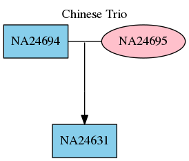
For more information about the PED file format see Pedigree PED input file format.
The VCF files output by the RTG pedigree-aware variant calling commands
contain full pedigree information represented as VCF header lines, and
the pedstats command can also take these VCFs as input. For example,
given a VCF produced by the population command after calling the
CEPH-1463 pedigree:
$ dot -Tpng <(rtg pedstats --dot "CEPH 1463" population-ceph-calls.vcf.gz) -o ceph-1463.png
Would produce the following pedigree directly from the VCF:
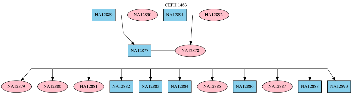
Note
Graphviz is provided directly via many operating system package managers, and can also be downloaded from their web site: https://www.graphviz.org/
See also
avrstats
Synopsis:
Print statistics that describe an AVR model.
Syntax:
$ rtg avrstats [OPTION]... FILE
Example:
$ rtg avrstats avr.model
Parameters:
Reporting |
||
|---|---|---|
|
Name of AVR model to use when scoring variants. |
|
Utility |
||
|---|---|---|
|
|
Print help on command-line flag usage. |
Usage:
Used to show some simple information about the AVR model, including when the model was built and which predictor attributes were employed during the model build.
See also
rocplot
Synopsis:
Plot ROC curves from readsimeval and vcfeval ROC data files, either
to an image, or using an interactive GUI.
Syntax:
$ rtg rocplot [OPTION]... FILE+
$ rtg rocplot [OPTION]... --curve STRING
Example:
$ rtg rocplot eval/weighted_roc.tsv.gz
Parameters:
File Input/Output |
||
|---|---|---|
|
ROC data file with title optionally specified (path[=title]). May be specified 0 or more times. |
|
|
If set, output a PNG image to the given file. |
|
|
If set, output a SVG image to the given file. |
|
|
Show a zoomed view with the given coordinates, supplied in the form <xmax>,<ymax> or <xmin>,<ymin>,<xmax>,<ymax> |
|
|
ROC data file. May be specified 0 or more times. |
|
Reporting |
||
|---|---|---|
|
If set, print rocplot command used in previously saved image. |
|
|
If set, hide the side pane from the GUI on startup. |
|
|
If set, interpolate curves at regular intervals. |
|
|
Sets the plot line width (Default is 2) |
|
|
Name of color palette to use. Allowed values are [blind_13, blind_15, blind_8, brewer_accent, brewer_dark2, brewer_paired, brewer_pastel1, brewer_pastel2, brewer_set1, brewer_set2, brewer_set3, classic] (Default is classic) |
|
|
If set, use a plain plot style. |
|
|
If set, show points on each curve. |
|
|
|
If set, plot precision vs sensitivity rather than ROC. |
|
If set, show scores on the plot. |
|
|
|
Title for the plot. |
Utility |
||
|---|---|---|
|
|
Print help on command-line flag usage. |
Usage:
Used to produce ROC plots from the ROC files produced by
readsimeval, bndeval and vcfeval. By default this opens the
ROC plots in an interactive viewer. On a system with only console access
the plot can be saved directly to an image file using the either the
--png or --svg parameter.
ROC data files may be specified either as direct file arguments to the
command, or via the --curve flag. The former method is useful when
selecting files using shell wild card globbing, and the latter method
allows specifying a custom title for each curve, so use whichever method
is most convenient.
Strictly speaking, a true ROC curve should use rates rather than absolute numbers on the X and Y axes (e.g. True Positive / Total Positives rather than True Positives on the Y, and False Positive / Total Negatives on the X axis). However, there are a couple of difficulties involved with computing these rates with variant calling datasets. Firstly, the truth sets do not include any indication of the set of negatives (the closest we may get is in the cases of truth sets which contain a set of confidence regions, where it can be assumed that no other variants may be present inside the specified regions); secondly even with knowledge of negative regions, how do you count the set of possible negative calls, when a call could occupy multiple reference bases, or even (in the case of insertions) zero reference bases. It is conceptually even possible to have a call-set contain more false positives than there are reference bases. For this reason the ROC curves are plotted using the absolute counts.
Precision/sensitivity (also known as precision/recall) curves are
another popular means of visualizing call-set accuracy, and these
metrics also do not require a count of Total Negatives and so cause no
particular difficulty to plot. Precision/sensitivity graphs can be
selected from the command line via the --precision-sensitivity flag,
or may be interactively selected in the GUI.
An interesting result of ROC analysis is that although there may be few
data points on an ROC graph, it is possible to construct a filtered
dataset corresponding to any point that lies on a straight line between
two points on the graph. (For example, using threshold A for 25% of the
variants and threshold B for 75% of the variants would result in
accuracy that is 75% of the way between the points corresponding to
thresholds A and B on the ROC plot). So in a sense it is meaningful to
connect points on an ROC graph with straight lines. However, for
precision/sensitivity graphs, it’s incorrect to connect adjacent points
with a straight line, as this does not correspond to achievable accuracy
on the ROC convex hull and can over-estimate the accuracy. Instead, we
can plot appropriately interpolated values with the --interpolate
option.
The default ROC graphs include some flourishes such as background
gradients and axes drop shadows, these can be disabled via the
--plain parameter. Alternative preset color palettes for the curve
colors may be selected with the --palette parameter, and in
particular some palettes are more color-blind friendly than the default
palette. In addition, PNG images saved by rocplot include metadata
indicating the graph configuration that may be useful when recreating
graphs. This metadata can be displayed (when present) via the --cmd
parameter.
Interactive GUI
The following image shows the rocplot GUI with an example ROC plot :
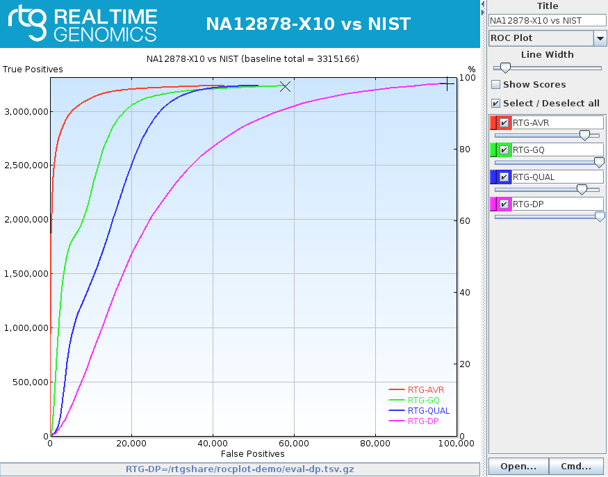
Similarly, here is an example precision/sensitivity plot:
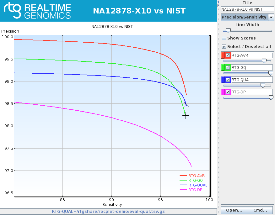
Some quick tips for the interactive GUI:
Select regions within the graph to zoom in. Right click within the graph area to bring up a context menu that allows undoing the zoom one level at a time, or resetting the zoom to the default.
The graph right click menu also allows exporting the image as PNG or SVG. (The saved image does not include the RTG banner).
Click on a spot in the graph to show the equivalent accuracy metrics for that location in the status bar. Clicking to the left or below the axes will remove the cross-hair. Note that sensitivity depends on the baseline total number of variants being correct. If for example the ROC curve corresponds to evaluating an exome call-set against a whole-genome baseline, this number will be inaccurate.
A secondary cross-hair is also available by holding down shift when placing (or removing) the cross-hair. When two cross-hairs are placed or moved, metrics in the status bar indicate the difference between the two positions.
Additional ROC data files can be loaded by clicking on the “Open…” button, and multiple ROC data files within a directory can be loaded at once using multi-select. Alternatively, you may use Drag and Drop from your file browser to drop ROC data files into either the graph area or the right hand ROC curve widget area.
The “Cmd” button will open a message window that contains a command-line equivalent to the currently displayed set of curves. This command-line may be copy-pasted, providing an easy way to replicate the current set of curves in another session, generate a curve in a script, or share with a colleague.
There is a drop down that allows for switching between ROC and precision/sensitivity graph types.
Each curve in the GUI has a customization widget on the right hand side of the window that allows several operations:
Rename the title used for the curve via the editable text.
Temporarily hide/show the curve via selection checkbox.
Reorder curves via drag and drop using the colored handle on the left.
Right click within the ROC widget area to bring up a context menu that allows permanently removing that curve, or customizing the color used for the curve
Each curve has a slider to simulate the effect of applying a threshold on the scoring attribute. If the “show scores” option is set, this provides an easy way to select appropriate filter threshold values, which you might apply to variant sets using
rtg vcffilteror similar VCF filtering tools.
Note
For definitions of the terminology used when evaluating caller accuracy, see: https://en.wikipedia.org/wiki/Receiver_operating_characteristic and https://en.wikipedia.org/wiki/Sensitivity_and_specificity
Note
For a description of the precision/sensitivity interpolation, see: “The relationship between Precision-Recall and ROC curves”, Davis, J., (2006), https://dx.doi.org/10.1145/1143844.1143874
See also
hashdist
Synopsis:
Counts the number of times k-mers occur in an SDF and produces a histogram. Optionally creates a blacklist of highly occurring hashes that can be used to increase mapping speed
Syntax:
$ rtg hashdist [OPTION]... -o DIR SDF
Parameters:
File Input/Output |
||
|---|---|---|
|
|
Directory for output. |
|
SDF containing sequence data to analyse. |
|
Sensitivity Tuning |
||
|---|---|---|
|
If set, output a blacklist containing all k-mer hashes with counts exceeding this value. |
|
|
Multiplier for the minimum size of the hash map (Default is 1.0) |
|
|
Soft minimum for hash count (i.e. will record exact counts of at least this value) (Default is 500) |
|
|
|
Step size (Default is 1) |
|
|
Number of bases in each hash (Default is 22) |
Utility |
||
|---|---|---|
|
|
Print help on command-line flag usage. |
|
Install the blacklist into the SDF for use during mapping. |
|
|
|
Number of threads (Default is the number of available cores) |
Usage:
Used to produce a text file containing a histogram of k-mer
frequencies. The --word parameter is used to select the width of the
k-mer and the --step parameter is used to select the distance
between successive k-mer start positions.
By specifying the --blacklist-threshold parameter a list k-mers
that occur more than the given number of times will be produced. Using
the --install-blacklist option will install the resulting blacklist
file into the specified SDF, which will permit use of the
--blacklist-threshold parameter of the map command.
The --max-count parameter can be used to inexactly adjust memory
requirements by setting a lower bound on the largest k-mer count that
will be recorded. For example, --max-count 500 will select a number
greater than or equal to 500 (exactly how much greater will depend on
other memory requirements), and will record exact frequencies for all
k-mers than occur less than this number. All k-mers that occur more
frequently than the chosen limit will be capped at the limit.
The --hashmap-size-factor parameter controls the default size of the
internal hash map, which in turn affects the RAM required to run the
command. This value may need to be increased if hashdist reports
warnings about too many hash collisions. Alternatively this parameter
could be reduced in order to run on a machine with lower RAM, but this
may reduce the likelihood that the command will complete successfully.
See also
ncbi2tax
Synopsis:
Converts the NCBI taxonomy into an RTG taxonomy for use in species database construction.
Syntax:
$ rtg ncbi2tax [OPTION]... DIR
Example:
$ wget ftp://ftp.ncbi.nlm.nih.gov/pub/taxonomy/taxdump.tar.gz
$ tar zxf taxdump.tar.gz -C ncbitaxdir
$ rtg ncbi2tax ncbitaxdir >rtg_taxonomy.tsv
Parameters:
File Input/Output |
||
|---|---|---|
|
Directory containing the NCBI taxonomy dump. |
|
Utility |
||
|---|---|---|
|
|
Prints help on command-line flag usage. |
Usage:
Used to create an RTG taxonomy file from an NCBI taxonomy dump. The
resulting taxonomy TSV file can be directly filtered with the
taxfilter command prior to creating a species reference SDF according
to project needs.
For more information on the RTG taxonomy format, and the associated sequence to taxon mapping file needed to create a species reference SDF, see RTG taxonomic reference file format.
taxfilter
Synopsis:
Provides filtering of a metagenomic species reference database taxonomy.
Syntax:
$ rtg taxfilter [OPTION]... -i FILE -o FILE
Example:
$ rtg taxfilter -P -i species-full.sdf -o species-pruned.sdf
Parameters:
File Input/Output |
||
|---|---|---|
|
|
Taxonomy input. May be either a taxonomy TSV file or an SDF containing taxonomy information. |
|
|
Filename for output TSV or SDF. |
Filtering |
||
|---|---|---|
|
|
When filtering an SDF, remove nodes below the first containing sequence data. |
|
|
When filtering an SDF, exclude sequence data from non-leaf output nodes. |
|
|
File containing ids of nodes to remove. |
|
|
File containing ids of nodes to remove sequence data from (if any). |
|
Assign a rank to “no rank” nodes from file containing id/rank pairs. |
|
|
|
File containing ids of nodes to include in subset. |
|
|
File containing ids of nodes to include as subtrees in subset. |
Utility |
||
|---|---|---|
|
|
Prints help on command-line flag usage. |
Usage:
The taxfilter command is used to manage metagenomic species
reference taxonomies and associated reference species SDF, primarily to
allow redundancy reduction and extraction of a subset of the database
according to project needs.
Building a metagenomic species database from all available data typically results in a very large database with high levels of redundancy, as often multiple strains of species are present, and often entire branches of the taxonomic structure are irrelevant for the project at hand. The following options provides methods to prune the taxonomy to sections of interest.
The --remove option will remove the specified taxon IDs from the
taxonomy (along with any child nodes), which can be used to exclude
entire subtrees of the full taxonomy. For example, you might exclude all
Proteobacteria by specifying that taxfilter should remove node with
taxon ID 1224.
The --subset option allows retaining only the specified list of
taxon IDs, along with any parent nodes required to reach the root of the
taxonomy. This would typically be used to specify a list of species or
strains of interest.
The --subtree option allows retaining the specified nodes, along
with their children and any parent nodes required to reach the root of
the taxonomy. For example, you could retain all Firmicutes by specifying
that taxfilter should keep the subtree with taxon ID 1239.
It is also often the case that ranks have not been fully assigned for
each node in the taxonomic structure. The --rename-norank option
allows manual rank assignment for any of these nodes for which rank
information can be obtained via other means, such as manual curation.
The species command requires that the reference database not contain
sequence data assigned to internal nodes of the taxonomy, so the
application of --prune-internal-sequences,
--prune-below-internal-sequences, or --remove-sequences may be
required before using any such database with the species command. The
taxstats command can be used to list the ids of internal taxons that
have sequence data attached.
Note that a quick way to extract all the genomic sequence associated
with a species (or multiple species) is to use the sdf2fasta command
with the --taxon flag.
taxstats
Synopsis:
Summarize and perform a verification of taxonomy and sequence information within a metagenomic species reference SDF.
Syntax:
$ rtg taxstats [OPTION]... SDF
Example:
$ rtg taxstats species-full.sdf
Warning: 340 nodes have no rank
214 nodes with no rank are internal nodes
126 nodes with no rank are leaf nodes
126 nodes with no rank have sequences attached
TREE STATS
internal nodes: 3724
leaf nodes:     5183
total nodes:    8907

RANK COUNTS
rank             internal leaf total
class                  58    0    58
family                300    0   300
genus                 940    1   941
no rank               214  126   340
order                 127    0   127
phylum                 34    0    34
species              1709 1703  3412
species group          34    0    34
species subgroup        7    0     7
strain                146 3347  3493
subclass                5    0     5
subfamily              17    0    17
subgenus                1    0     1
suborder               19    0    19
subphylum               1    0     1
subspecies            104    6   110
superkingdom            3    0     3
superphylum             3    0     3
tribe                   2    0     2
TOTAL                3724 5183  8907

SEQUENCE LOOKUP STATS
total sequences:           309367
unique taxon ids:            5183
taxon ids in taxonomy:       5183
taxon ids not in taxonomy:      0
internal nodes:                 0
leaf nodes:                  5183
no rank nodes:                126
Parameters:
File Input/Output |
||
|---|---|---|
|
SDF to verify the taxonomy information for. |
|
Reporting |
||
|---|---|---|
|
List details of sequences attached to internal nodes of the taxonomy. |
|
Utility |
||
|---|---|---|
|
|
Prints help on command-line flag usage. |
Usage:
The taxstats command outputs statistics regarding the contents of a
metagenomic species reference database, in order to indicate the number
of members of each rank, and how many have sequence information
contained within the database.
Any discrepancies found within the database will be issued as warnings.
usageserver
Synopsis:
Start a local network usage logging server.
Syntax:
$ rtg usageserver [OPTION]...
Example:
$ rtg usageserver
Parameters:
Utility |
||
|---|---|---|
|
|
Prints help on command-line flag usage. |
|
|
Set this flag to change which port to listen for usage logging connections. (Default is 8080). |
|
|
Set this flag to change the number of threads for handling incoming connections. (Default is 4). |
Usage:
Use the usageserver command to run a usage logging server for a local
network. For more information about usage logging and setup see
Usage logging
version
Synopsis:
The RTG version display utility.
Syntax:
$ rtg version
Example:
$ rtg version

Product: RTG Core 3.9
Core Version: 718f8317b7 (2018-05-29)
RAM: 25.0GB of 31.3GB RAM can be used by rtg (79%)
CPU: Defaulting to 4 of 4 available processors (100%)
JVM: Java HotSpot(TM) 64-Bit Server VM 1.8.0_161
License: Expires on 2019-05-20
Contact: support@realtimegenomics.com

Patents / Patents pending:
US: 7,640,256, 9,165,253, 13/129,329, 13/681,046, 13/681,215, 13/848,653, 13/925,704, 14/015,295, 13/971,654, 13/971,630, 14/564,810
UK: 1222923.3, 1222921.7, 1304502.6, 1311209.9, 1314888.7, 1314908.3
New Zealand: 626777, 626783, 615491, 614897, 614560
Australia: 2005255348, Singapore: 128254

Citation (variant calling):
John G. Cleary, Ross Braithwaite, Kurt Gaastra, Brian S. Hilbush, Stuart Inglis, Sean A. Irvine, Alan Jackson, Richard Littin, Sahar Nohzadeh-Malakshah, Mehul Rathod, David Ware, Len Trigg, and Francisco M. De La Vega. "Joint Variant and De Novo Mutation Identification on Pedigrees from High-Throughput Sequencing Data." Journal of Computational Biology. June 2014, 21(6): 405-419. doi:10.1089/cmb.2014.0029.

Citation (vcfeval):
John G. Cleary, Ross Braithwaite, Kurt Gaastra, Brian S. Hilbush, Stuart Inglis, Sean A. Irvine, Alan Jackson, Richard Littin, Mehul Rathod, David Ware, Justin M. Zook, Len Trigg, and Francisco M. De La Vega. "Comparing Variant Call Files for Performance Benchmarking of Next-Generation Sequencing Variant Calling Pipelines." bioRxiv, 2015. doi:10.1101/023754.

(c) Real Time Genomics, 2025
Parameters:
There are no options associated with the version command.
Usage:
Use the version command to display release and version information.
license
Synopsis:
The RTG licensed commands display utility.
Syntax:
$ rtg license
Example:
$ rtg license
Parameters:
There are no options associated with the license command.
Usage:
Use the license command to display the release status of each licensed
command. Output at the command line (standard output) shows command name,
licensed status, and command release level.
help
Synopsis:
The RTG help command provides online help for all RTG commands.
Syntax:
List all commands:
$ rtg help
Show usage syntax and flags for one command:
$ rtg help COMMAND
Example:
$ rtg help format
Parameters:
There are no options associated with the help command.
Usage:
Use the help command to view syntax and usage information for the main
rtg command as well as individual RTG commands.